Message Boards Message Boards

0
|
7811 Views
|
6 Replies
|
4 Total Likes
View groups...
Share
Share this post:

Upper and lower bounds of data

Posted 9 years ago

Hi everyone,

I have sets of points and I would like to find functions that are uppuer/lower bouds of them. It is not the fitting curve, it is the closest curve that all the points are above/below it. It is important to say that I have no idea of how doing it. My first thought was using some kind of least square routine, but I am not sure if I can do it.

Well, I would be thankful if someone have any ideas.

POSTED BY: patrick
6 Replies
Posted 9 years ago

Thanks for all your helpin and suggestions, Marco!

I understand what you are saying, but I have something different in mind, and I think I have a different problem, too. It is difficult for me to tell you what exactly is my problem, but I think we are going in a good way!

Let's say my data has all the maxima points for 50 random plots I did. Then I increase it for 200, 500 or 1000 plots and as I increase then number of functions, my maxima points increases too, but it'll converge to a specific curve which all points of my data would be =< comparing to the points of this function. By the theory I have, it must to be like "a+bCos[x]^2", and I "guess" that the best upper bound I would have is 1/2(1+Cos[x]^2), but I want a consistend proof of it, not just a guess -- well, I could use this guess for my data, but other than that I have some strange curves and I would not be that easy to find the upper bound function by guess. I want an algorithm that would give my this upper (or lower) bounds for my data.

The best idea I have, but I cannot implement it, is by using the least squares method with a constraint that the difference between the points of my upper bound function and my data must be positive. Then I try to minimize it and find find the parameters. Then I increase the points and see that (maybe) it'll converge to 1/2*(1+Cos[x]^2). Do you think it is possible to do it and that it is the best way find what I want? The thing is that my points don't have to necessarily be equal to the upper bound function ones, they just have to be bellow it.

I think that's it. Thanks for the help!

Cheers

POSTED BY: patrick

Hi Patrick,

ok, I can see the problem now. I have a very different suggestion that involves the new and experimental function FindFormula. I must admit that this is an absolutely magic function for me, but it is very useful. In your example you have the data in the variable A and you "guess" the function that should approximate the data. Your guess is of the form:

a + b*(Cos[\[Theta]])^2 

Now, in general we don't know that and also FindFormula is able to find a much better approximation. After your parameter estimation you get something like this:

enter image description here

Now, let's try what FindFormula does:

FindFormula[A][x]

enter image description here

Looking at this shows that the polynomial approximation is surprisingly good.

Show[ListPlot[A], Plot[FindFormula[A][x], {x, 0, 1.6}]]

enter image description here

It is practically impossible to see deviations. Now let's try to find upper and lower bounds.

eqn = FindFormula[A][x];
deviation = Max[Abs[((eqn /. x -> #[[1]]) - #[[2]])] & /@ A];
Show[ListPlot[A], Plot[{eqn, eqn + deviation, eqn - deviation}, {x, 0, 1.6}]]

enter image description here

The important bit is the deviation formula. It looks for the largest deviation of all data points from the estimated curve. The figure contains four curves: the data, the estimated equation, the upper and the lower bound. You can be sure that the upper and lower bounds are larger/equal and lower/equal to the deviations.

I think that the crucial point is when you say "and it fits well with the following function". If you have any reason to believe that this should be the function to fit (i.e. you have a theory that tells you so) then you can proceed like you did. If you do not have a theory and just want a good upper/lower bound you might want to do what I suggest. Also, you could of course look for deviations from the eqn separately for points that are higher and the ones that are lower. You would get one of the two estimates slightly closer to eqn.

Does this help?

Cheers,

Marco

PS: The following is unrelated to your problem, but I hope it illustrates what I mean by magic. Suppose you have data from a sin function and apply FindFormula:

formula = FindFormula[Table[Sin[0.1 x] + 0.2, {x, 1, 100}]][x]

This gives:

enter image description here

which looks really horrible. Nothing at all like a Sine function; there is a Log function in there and we obtain a weird piecewise function. Now the magic is this:

Plot[{Sin[0.1 x] + 0.2, formula}, {x, 0, 100}]

enter image description here

which is utterly surprising for me. That strange piecewise function is a very accurate representation of the sin function in that interval. I would really like to see how the Wolfram Language comes up with that! If someone of the Wolfram team could comment on this and indicate what is going on, that would be really interesting.

POSTED BY: Marco Thiel
Posted 9 years ago

Marco,

I just add a file with my data and I try to explain what I want in the file. Please, if you have any guess, I would be thankful.

Cheers.

Patrick

Attachments:
POSTED BY: patrick

Hi Patrick,

can you post the data an graphic of what you want to achieve or have achieved?

Cheers,

Marco

POSTED BY: Marco Thiel
Posted 9 years ago

Hi Marco,

Thanks for your answer. I think I should be more pricise in my question, as you said. The thing is that I have some random values, I found their maxima (and minima), and I want to find the curve(s) that is(are) upper(lower) bound of this(these) maxima(minima). By using "FindFit", I can have an idea of what I am looking for, but I want that all the points must be below/above the curves.

POSTED BY: patrick

Hi,

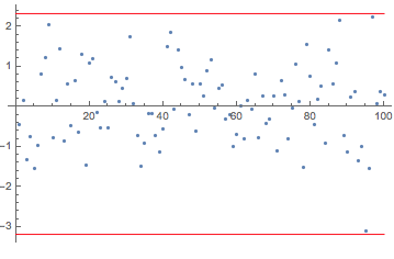
I am not sure whether I understand your question. If you have data and you take the max and the min you would get upper and lower bounds.

data = RandomVariate[NormalDistribution[], 100]; \[Epsilon] = 
 0.1*Variance[data];
ListPlot[data, 
 Epilog -> {Red, 
   Line[{{0, Max[data] + \[Epsilon]}, {Length[data], 
      Max[data] + \[Epsilon]}}], Red, 
   Line[{{0, Min[data] - \[Epsilon]}, {Length[data], 
      Min[data] - \[Epsilon]}}]}]

enter image description here

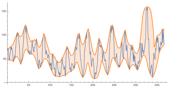
I believe that this technically solves your problem. I generate two curves, which bound the time series. But this appears to be too easy to be your problem. So probably your are interested in something they call "the envelop". Perhaps this post helps you. You might also like this demonstration, which contains this piece of code:

Manipulate[
 ListLinePlot[{data, 
   EstimatedBackground[data, \[Sigma], 
    Method -> {"SNIP", r}], -EstimatedBackground[-data, \[Sigma], 
     Method -> {"SNIP", r}]}, AspectRatio -> 1/2, ImageSize -> Medium,
   PlotStyle -> {Automatic, {Orange, Thick}, {Orange, Thick}}, 
  Filling -> {2 -> {3}}], {{\[Sigma], 10}, 2, 30, 1}, {r, 0, 20},
 Initialization :> (data = 
    WolframAlpha[
      "sunspot", {{"SunspotsPartialTimeSeries:SpaceWeatherData", 1}, 
       "TimeSeriesData"}][[All, 2]])]

enter image description here

This suggests that you need to be more specific regarding your objective. There are parameters in here ("how smooth do I want the envelope to be?"), which need to be included in the original question.

Note that the core of the animation is the EstimatedBackground function which is new in MMA10.

ListLinePlot[{data, 
  EstimatedBackground[data, 5, 
   Method -> {"SNIP", 0.1}], -EstimatedBackground[-data, 5, 
    Method -> {"SNIP", 0.1}]}, AspectRatio -> 1/2, ImageSize -> Large,
  PlotStyle -> {Automatic, {Orange, Thick}, {Orange, Thick}}, 
 Filling -> {2 -> {3}}]

enter image description here

I hope that this helps you to find a solution to your problem.

Cheers,

Marco

POSTED BY: Marco Thiel
Reply to this discussion
Community posts can be styled and formatted using the Markdown syntax.
Reply Preview
Attachments
Remove
or Discard

Group Abstract Group Abstract