I find something in my calculation that may not be delivering what is needed. The image data has a wedge which is biasing the calculation:

Here the centroid and radius of the annulus is marked:

Here you can see the wedge:

It may be possible to solve this by clipping the data, or by de-wedging by subtracting a best-fit plane. The attached notebook displays this, but does not attempt to correct it.

Attachments:

Hi Antonio,

Yes, the second part is still connected, and the symbol "files" has a value which is the list of file names. I reused the name "files" in the argument to the analyzeImageGroup function, which was a bit confusing. But appearing as an argument it is a formal parameter, and not the same. The function accepts a list of file names, which are still available as the value of the global symbol "files." But when used, analyzeImageGroup just expects a list of file names, each being a string. In the notebook, these are given without full paths because we have already set the default directory to the notebook directory, and the files are in it.

Here is some code which was executed after the notebook was executed. Notice that files still has a value which is our full list of file names. But I can also give the function a list of file names I have typed in. And I can also Map the function onto a list of lists, where each bottom level list is a list of file names. Now I get a list of analysis results, one result for each of the bottom level list of file names. This could be used to process an entire set of data, consisting of separate lists for each group of images which should be added and analyzed.

In[63]:= files

Out[63]= {"fiber3_0.fits", "fiber3_1.fits", "fiber3_2.fits", \
"fiber3_3.fits", "fiber3_4.fits"}

In[64]:= analyzeImageGroup[files]

Out[64]= {{476.983, 500.031}, 386.469, {"fiber3_0.fits", 
  "fiber3_1.fits", "fiber3_2.fits", "fiber3_3.fits", "fiber3_4.fits"}}

In[65]:= (* Here we explicitly give it a list of file names *)

In[66]:= analyzeImageGroup[{"fiber3_1.fits", "fiber3_2.fits"}]

During evaluation of In[66]:= InterpolatingFunction::dmval: Input value {0.652631,498.308} lies outside the range of data in the interpolating function. Extrapolation will be used. >>

During evaluation of In[66]:= InterpolatingFunction::dmval: Input value {0.176204,498.308} lies outside the range of data in the interpolating function. Extrapolation will be used. >>

During evaluation of In[66]:= InterpolatingFunction::dmval: Input value {-0.300222,498.308} lies outside the range of data in the interpolating function. Extrapolation will be used. >>

During evaluation of In[66]:= General::stop: Further output of InterpolatingFunction::dmval will be suppressed during this calculation. >>

Out[66]= {{471.156, 498.285}, 387.422, {"fiber3_1.fits", 
  "fiber3_2.fits"}}

In[67]:= (* The errors are not a problem, but can be turned off if we \
want *)

In[68]:= Off[InterpolatingFunction::dmval]

In[69]:= analyzeImageGroup[{"fiber3_1.fits", "fiber3_2.fits"}]

Out[69]= {{471.156, 498.285}, 387.422, {"fiber3_1.fits", 
  "fiber3_2.fits"}}

(* We can Map the function onto a list of lists to get a list of \
results *)

In[70]:= listOfLists = {{"fiber3_1.fits", 
    "fiber3_2.fits"}, {"fiber3_3.fits", "fiber3_4.fits"}};

In[71]:= analyzeImageGroup /@ listOfLists

Out[71]= {{{471.156, 498.285}, 
  387.422, {"fiber3_1.fits", "fiber3_2.fits"}}, {{473.682, 500.875}, 
  386.866, {"fiber3_3.fits", "fiber3_4.fits"}}}

(* Turn the error message back on *)

Hi Antonio,

Just about the first line in the notebook uses FileNames function to generate a list of the file names as strings and assign the list to the symbol files. But any method that generates such a list would work the same. You could also Map the analysis function onto a list of lists to analyze severa groups of files.

Yes. I would love to see the paper. You could attach it or send it to my email.

Best, David

Hi Antonio, How this happens depends on which plotting function you use to display the image. Mathematica ListPlot and ContourPlot and similar functions plot f[x,y] with x on the horizontal and y on the vertical, increasing left to right and bottom to top as usual. But ArrayPlot and similar functions plot array[[row,column]] with rows on the vertical axis, increasing top to bottom, and columns on the horizontal, increasing left to right. (Edit: It looks like the graphic of an image, as when it is first imported, is oriented like the graphic plotting routines, not like ArrayPlot.)

So if we build an interpolating function with the row and column indices in the x and y position we get this rotation, and ListInterpolation will do this.

temp = {
   {1, 1, 0, 0, 0},
   {1, 1, 0, 0, 0},
   {0, 0, 0, 0, 0},
   {0, 0, 0, 0, 0},
   {0, 0, 0, 0, 0}};

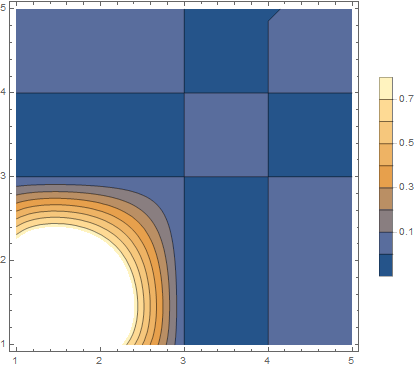
tf = ListInterpolation[temp];

ContourPlot[tf[x, y], {x, 1, 5}, {y, 1, 5}, PlotLegends -> Automatic]

This could be overcome by building the Interpolating function differently. Also, ArrayPlot has an option that helps. (Note that ArrayPlot inverts intensity to create a negative image.) Here Transpose swaps rows for columns, and DataReversed plots bottom to top.

ArrayPlot[temp // Transpose, DataReversed -> True]

Best,

David

Hi Antonio, I looked at the file I sent earlier (Cesar 1_2.nb) and used Get Coordinates on the original summed image. I can't say my guess at a center was good, but when I put the cursor at the center determined by the algorithm I get matching values. What are you seeing?

Best, David

PS: What makes the ring?

Get Coordinates:

The calculated center:

Hi Antonio,

I think convergence will be influence by the image data. With sufficiently noisy the process could just wander around. A choice of a center produces a set of maxima, which produces a different center, etc. There could be patterns that even cycle without convergence. For sufficiently noisy image data we might be just wandering until we happen to get 2 centers in a row which are sufficiently close. But the process really doesn't converge in a continuous way. It might converge better for smoothed data, but then you have to ask if that particular converged result is really better than one of the results from acting on non-smoothed data.

I was looking at a different calculation which might be interesting. I calculate the set of maxima around the ring as before. But instead of calculating a center from the XY positions, I use the XYZ positions and fit to a plane. The Z is the image intensity. It is interesting the way the ring is sharp and intense toward one side, and broader and less intense toward the other. One possible explanation is that it is as an object more uniform, but in the imaging system it is tilted with respect to the optical axis -- so the broader less intense side is really just out of focus.

This "tilt" is of course just a parameter. The X and Y is in units of pixels (which are distance), and the Z is in intensity, which is in different units, so ArcTan of intensity divided by distance is a rather strange thing.

Here is a code snippet. It calculates a tilt of almost 1 degree for the plane fitting the maxima:

In[33]:= fit = LinearModelFit[centeredMaxima, {x, y}, {x, y}];

In[34]:= parameters = fit["BestFitParameters"]

Out[34]= {-2.91103*10^-17, 0.00012698, -0.00154588}

In[35]:= tilt = Norm[parameters[[{2, 3}]]]/Degree

Out[35]= 0.0888707

In[36]:= fitFunction = fit["BestFit"]

Out[36]= -2.91103*10^-17 + 0.00012698 x - 0.00154588 y

Here is a set of maxima and the best fit plane:

Hi David, I need more time to evaluate your latest code. So far I could take apart and understand your previous code almost completely. I have not a final conclusion yet. I can say that the code seems to work as it should and that their algorithm seems ok. However, I'm not too sure about the result, I need to continue investigating. Give me some more days......

This experiment is not confidential, You can ask what you want. This is a situation in which light from a laser is incident on the input fiber with an angle to the surface. The result is that the output light is a ring-shaped projection. The image that you see, is obtained with the help of a beam spliter reflecting the ring projected onto a target at about 1 meter from the output of the fiber. The analysis of the results can give us informations about the polishing angle of the fiber in test.

Thanks a lot.....

Best regards,

Antonio

Hi Antonio,

The code I posted yesterday uses an algorithm like you first described -- it determines a point "centered" with respect to a collection of maxima along radials, and it iterates. It may work.

Regarding the addition of a list of images, that is what it does. You give it a list of file names. It imports those files as images, adds them to make one image, and analyzes it. This can be immediately extended as you describe above. If you partition the file names into a list of lists, where each low level list is a list of files you want added and analyzed, then you will get a list of results. Look at the function named Map. Map[f,{a,b,c}] outputs { f[a], f[b], f[c] }.

So if you have a large list of files which you want to be analyzed in groups, you partition them:

partitionedFiles = { {file1, file2, file3, file4, file5}, {file6, files6, file8, file9, file10} }

And then

Map[ AnalyzeImageGroup, partitionedFiles]  or the shortcut AnalyzeImageGroup/@partitionedFiles

will produce an analysis for each of the sublists as a group. You will get a list of results, one result for each group. And an annotated graph will be saved as a png for each of the groups, using the name of the first file in the group for the name of the png.

Kind regards,

David

Hi Cesar,

Yes -- transitioning from procedural structures is always difficult at first. And I still find that there are some cases where I feel a procedural structure would be better. But they are very few.

Mathematica uses a functional paradigm in a way which is more functional than even C or Fortran. When I need to perform a repeated function like performing the same process on different groups of images, I write a function. The function accepts a list of images, there could be any number, and performs the entire analysis. It could just output numbers, like the centroid, or it could export images and graphs as part of the evaluation.

I don't try to write the function immediately. I work in a notebook, like we are doing with this. Then, once the method works, I "glue" the cells together into a sequence of statements separated by semicolons, and add the functional head and closing bracket. The functional head includes the argument(s), and often employs Module for encapsulation. This is easier than it sounds. Once the sequence of cells work, I terminate each with a semicolon, evaluate again to get rid of the output cells, and use Cell/Merge to join them in a single cell.

The final result here would be a function that accepts a list of files or images, then acts on them. We could take a bunch files in a list, partition it into the groups that should be analyzed separately, and then Map the function onto the list of lists. The result is a list of the evaluation results for each group which was in its own list.

I am still thinking about the method I used. It appears that the image has a wedge in the focus -- that is the focal plane is tilted with respect to the imager. This makes the ring higher and narrower on the in focus side, and shorter and fatter on the out of focus side. That may be the reason the circle representing the radial max does not align well with the image. It may be that your method of finding the maxima on lines is better. I'm still thinking about that.

Kind regards, David

Hi Antonio,

What I understand is that you wish to calculate the centroid of the image, and then perhaps the mean radial distance from the centroid to the annular ring. The attached notebook uses the usual normalized weighted sum to get the centroid, and then reprocesses the data into a purely radial dependency. From that it extracts the radius of the annulus. Note that I deleted the output cells to shrink the file for posting.

Some of the code may be a little difficult at first if you're just starting with Mathematica. But time spent learning Mathematica will be repaid many times. Here are two nice resources: An Elementary Introduction and Virtual Book

If I am not understanding this correctly, please let me know.

Kind regards,

David

Attachments:

Dear Frank, Thanks for your suggestion. I have a tendency to use looping because my only computer training was over 30 years with FORTRAN and looping was a very reasonable option. I will work hard with your suggestion ......... Thanks

Please attach a sample image. It will help in understanding.

Best regards, David

Initially I would like to apologize for this question involving a so large code. I am no expert in Mathematica and have been trying to learn from limited resources. I have been involved with this code longer than it should and that makes me really discouraged.From the moment I posted the code here I get some progress to find the center of a single image. This was achieved by using a looping type (Goto). My difficulty now is define another loop to redo the operations for the other images imported on begin of the code. I would really appreciate some help to finish this code to obtain the final value of the center of mass coordinates. Thanks for any help...

Attachments: