Over at reddit, some excellent questions/ observations were made.
- God, for a second I thought it was a sphere.
- Is there a formal proof that it has constant width?
For the first, what does happen when we compare this with a sphere? The caltrop-based surface of constant width will be done in yellow, and a sphere of radius .5 in blue. It's quite odd what happens.
Graphics3D[{{Yellow,ConvexHullMesh[Join[cal76,Flatten[is76scw,1]]]["GraphicsComplex"]},{Blue, Sphere[{0,0,0}, .5]}},Boxed->False,ViewAngle->Pi/10,ImageSize->{600,600}]
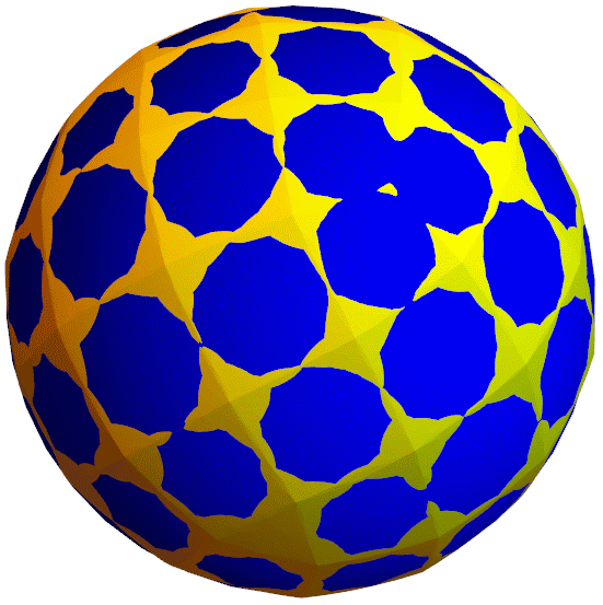
For the second, how can this be verified? I have a decent method in my post -- generate a lot of points, and find the farthest point from each point. If the farthest point is always at distance one as the number of random surface points gets arbitrarily large, then the solution works. I applied that method to the Resnikoff surface. But not to my own surface. On my own surface, I did a weaker check. That was rather presumptuous of me. The program I used for picking points at distance 1 was flawed. It was -- get a random point, find the farthest point in a pointset, move the point to distance 1. But the farthest point could change in the process of moving. Here's more careful code.
randomUnitDistancePointPolar[pointset_]:=
Module[{k,randomspherepointPositive, randomspherepointNegative,farpointsPositive, farpointsNegative,multiplierPositive,multiplierNegative },
randomspherepointPositive= coord[{RandomReal[{0,2Pi}],RandomReal[{-1,1}],1}];
randomspherepointNegative = -randomspherepointPositive;
farpointsPositive =  FarthestPoints[pointset,randomspherepointPositive,4];
farpointsNegative =  FarthestPoints[pointset,randomspherepointNegative,4];
multiplierPositive = Last[Sort[k/.Solve[{MyEuclidean[k  randomspherepointPositive,#]==1}]]]&/@farpointsPositive;
multiplierNegative = Last[Sort[k/.Solve[{MyEuclidean[k  randomspherepointNegative,#]==1}]]]&/@farpointsNegative;
{Sort[Table[{Max[Table[MyEuclidean[multiplierPositive[[k]]  randomspherepointPositive,farpointsPositive[[j]]],{j,1,4}]], multiplierPositive[[k]]  randomspherepointPositive},{k,1,4}]][[1,2]],
Sort[Table[{Max[Table[MyEuclidean[multiplierNegative[[k]]  randomspherepointNegative,farpointsNegative[[j]]],{j,1,4}]], multiplierNegative[[k]]  randomspherepointNegative},{k,1,4}]][[1,2]]}
];
Here are the 76 points.
cal76={{-0.4083582798988096`,-0.2742546402707427`,-0.09034731123170289`},{-9.958465404071062`*^-9,0.14648426006691528`,0.4782019350351851`},{6.73274361415451`*^-9,0.4020250213642393`,-0.2975073298522745`},{0.4083582831245314`,-0.2742546411604119`,-0.09034729395120787`},{-0.46005112774248885`,0.19669672299517796`,0.06479750202204874`},{-0.37646381006368895`,0.2828182459595357`,0.18117449242974917`},{-0.37646380664714646`,0.335125174376982`,0.02239368272554362`},{-0.08358732592409791`,-0.4267626938092579`,0.2557774801658645`},{-8.245298000993142`*^-9,-0.3406411708449002`,0.37215447057356493`},{0.08358731417059766`,-0.42676269399136524`,0.25577748370302866`},{0.37646380301309024`,0.2828182451393534`,0.18117450836056592`},{0.3764638064296328`,0.33512517355679966`,0.0223936986563603`},{0.46005112542898596`,0.19669672199288823`,0.0647975214900296`},{-0.08358731053654152`,-0.19118072552497012`,-0.45934567478913835`},{1.0558800920201747`*^-8,-0.05275227414316607`,-0.5017494940856435`},{0.0835873295581541`,-0.19118072570707753`,-0.45934567125197423`},{-0.13399475927338292`,0.3401518113710143`,-0.3479610215959084`},{3.935963916780783`*^-9,0.478209035807638`,-0.16140272895373037`},{0.13399475688050796`,0.06673824586943174`,0.48200221421544004`},{0.3029245473152117`,-0.38342759987801794`,-0.12631198330894344`},{-0.4369193136085767`,-0.24537037448950066`,0.060246290844122634`},{-0.43691930813168356`,-0.1615196817990518`,-0.19428750195276642`},{-0.3029245428054219`,-0.3834275992180518`,-0.12631199612779967`},{-0.1339947771319936`,0.06673824616135929`,0.48200220854518433`},{-8.445753645264267`*^-9,0.2886461632884318`,0.41402670839047334`},{0.1339947747391187`,0.3401518110790869`,-0.3479610159256526`},{0.4369193105245585`,-0.2453703754413943`,0.060246309333234584`},{0.4369193160014517`,-0.16151968275094553`,-0.1942874834636544`},{0.19857232806547456`,0.2414884119962342`,0.39691559128602183`},{-0.3014276658828522`,-0.39793238086123595`,0.07797943132815037`},{-0.19857234433563078`,0.24148841242885352`,0.39691558288303747`},{0.1985723403860086`,0.4301145723332891`,-0.17567040020422556`},{-0.4999999995937601`,-0.06907794446944336`,-0.022756256323355057`},{-0.1985723320150967`,0.4301145727659085`,-0.17567040860720995`},{-1.0624722918507781`*^-8,-0.08736602396293898`,0.49765127053454294`},{9.81224354438672`*^-9,0.2255219139911501`,-0.4521387790463301`},{0.30142766171604196`,-0.3979323815179409`,0.07797944408366307`},{0.30142766983247427`,-0.27367060390090675`,-0.29922461400696254`},{-0.3014276577664199`,-0.27367060324420184`,-0.29922462676247524`},{0.5000000004062395`,-0.06907794555876769`,-0.022756235164857957`},{-0.4779171238955934`,0.02608392988012896`,0.16331449187242988`},{-0.3660857189235138`,0.30324695712170446`,-0.17256680260947826`},{0.1469531522570092`,0.07747070721983303`,-0.47766079233150865`},{0.25878454841831394`,-0.10773258907155243`,-0.42092875729515894`},{0.47791711704144224`,0.026083928838915534`,0.16331451209644585`},{-0.3660857295010557`,0.1413058351635909`,0.31901515884135884`},{-0.25878454580394866`,-0.33682020241617083`,0.2744803855716309`},{-0.25878453084058534`,-0.10773258850775182`,-0.42092876824614284`},{-0.2191325810215751`,0.4546554290281564`,0.03203318211204315`},{-0.146953151409411`,-0.2215982971327089`,0.4301810525405597`},{-0.11183139061700911`,-0.35110079192819443`,-0.3463794825711219`},{0.11183139555301191`,-0.4882286748864234`,0.06988041180109335`},{0.11183140450982235`,-0.3511007921718357`,-0.3463794778387532`},{0.14695313272265692`,-0.22159829745286824`,0.43018105875917506`},{0.21913258065656127`,0.45465542855074365`,0.03203319138507527`},{0.25878453345495067`,-0.33682020297997145`,0.27448039652261474`},{0.3660857163091486`,0.14130583436601876`,0.3190151743330062`},{0.36608572688669044`,0.3032469563241323`,-0.17256678711783088`},{-0.4779171178890406`,0.11804366107396037`,-0.11583477230549717`},{-0.2191325855925641`,0.3846740382638743`,0.24446587938495315`},{-0.14695313187505868`,0.07747070753999229`,-0.47766079855012394`},{-0.11183139957381949`,-0.48822867464278213`,0.06988040706872475`},{0.21913257608557227`,0.3846740377864614`,0.2444658886579853`},{0.4779171230479952`,0.1180436600327469`,-0.11583475208148117`},{-0.407514327993345`,-0.16976437931749935`,0.24910041749277848`},{-5.161330127384547`*^-9,0.43139871213507613`,0.2661466534980246`},{0.2897103239985093`,-0.048388805251119736`,0.41311661996952853`},{0.2897103406552224`,0.20662382688011618`,-0.3609894772467069`},{0.40751431708230673`,-0.16976438020532986`,0.2491004347375597`},{-0.4075143161517443`,0.011529357945156408`,-0.301227565200711`},{-0.28971034158578496`,-0.04838880461994275`,0.4131166077098581`},{-0.28971032492907184`,0.20662382751129316`,-0.3609894895063774`},{-0.11780398699190484`,-0.4682581594410395`,-0.15425759872920716`},{-3.4621769187396477`*^-10,0.5051176070036564`,0.04236853897527871`},{0.11780399249945263`,-0.46825815969769297`,-0.15425759374409645`},{0.4075143289239075`,0.011529357057325836`,-0.30122754795592976`}};
Now we can generate 20000 random points and their polar opposites. This takes awhile to run. Then we combine them with the original 76 to get a checklist of 40076 points. For each point, we can find the distance to the farthest point. If there are any flaws, we can pick out the points that generated a distance over 1. Then we can get a minmax of the distances to see how bad the errors are, if any exist.
is76scw=Monitor[Table[randomUnitDistancePointPolar[cal76],{jj,1,20000}],jj];
check76 = Join[cal76, Flatten[is76scw, 1]];
dists=Monitor[Table[EuclideanDistance[check76[[k]],FarthestPoints[check76,check76[[k]],1][[1]]],{k,1,Length[check76]}],k];
bad = check76[[Flatten[Position[Sign[Chop[dists - 1]], 1]]]];
MinMax[dists]

{1., 1.00002}
Looks like some pairs of points can be a micron to far apart. Out of the 40076 points generated and the 803022850 possible pairs, here are the 50 points that can generate a distance of 1.000002 with some other point in the "bad" list.
bad = {{0.217299,0.453677,0.00289042},{0.21081,0.313122,0.327902},{-0.30425,-0.397356,0.0198628},{-0.305056,-0.396024,-0.00758598},{0.0769693,-0.491524,0.0703061},{0.499554,-0.0557945,0.003875},{0.0000341373,0.335519,0.371979},{-0.182439,-0.460237,0.0734066},{-0.15309,0.325789,-0.351062},{-0.421063,-0.266799,0.0628566},{0.316308,0.174691,0.346821},{0.262122,-0.118299,-0.414443},{-0.155536,0.323949,-0.351397},{-0.269515,-0.0325779,0.424797},{-0.0608613,0.167056,-0.467461},{0.324612,0.156324,-0.348921},{-0.332738,0.259147,-0.268588},{0.376774,0.333399,0.00612808},{0.247323,-0.0868552,-0.429567},{0.365602,0.0904816,-0.329314},{0.374647,0.0745269,-0.324088},{-0.0775596,0.150317,-0.470526},{0.16768,-0.243541,0.405892},{0.284112,-0.195228,-0.362151},{-0.334145,-0.0915662,0.361428},{0.295381,-0.276727,-0.301267},{-0.0000968207,0.504594,0.0277361},{0.127589,-0.204336,0.441693},{-0.280701,-0.283995,-0.306032},{0.465323,0.144349,-0.124355},{0.0174747,-0.355603,-0.350556},{-0.295778,-0.245216,-0.323275},{0.292672,-0.303975,0.27156},{-0.378837,-0.137164,0.29839},{0.21301,0.277084,-0.358325},{-0.0950728,0.132381,-0.473214},{-0.213059,0.329729,0.310047},{-0.352811,-0.0363017,-0.353029},{0.247033,0.436895,0.0305884},{-0.174493,-0.250587,0.397601},{-0.484321,0.0887515,-0.101515},{0.228601,0.410957,-0.176389},{-0.331244,0.164913,0.339026},{-0.430212,-0.218733,0.132927},{-0.473575,0.113459,0.114474},{-0.267608,-0.34923,0.243012},{-0.340969,-0.0984442,0.352577},{0.333913,0.0509263,0.368648},{0.485222,-0.0979485,-0.0753553},{-0.432159,-0.224615,0.117287}};
We can take a look at where these points are located in relation to the original 76 points.
Graphics3D[{{Opacity[.6],ConvexHullMesh[cal76]["GraphicsComplex"]},Table[Line[{FarthestPoints[bad,bad[[n]],1][[1]],bad[[n]]}],{n,1,Length[bad]}]},Boxed->False,ViewAngle->Pi/10,ImageSize->{600,600}]
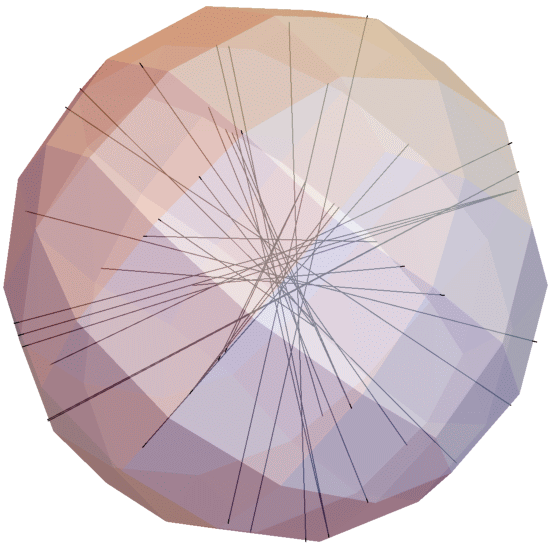
All of these bad point pairs connect an edge point to an edge point. For future checks, I can focus on those. There is plenty of play in the given caltrop, currently I'm optimizing for volume. How might I optimize for the edges working just slightly more nicely with each other? One method might be canonicalization. Here's some code adapted from George Hart's Canonical Polyhedra page.
view[v_, f_] :=
Graphics3D[{Opacity[.7],Polygon /@ Map[v[[#1]] & , f, {2}]}, SphericalRegion-> True,Boxed -> False]
face2edges[face_] := MapThread[Sort[{#1, #2}] & , {face, RotateLeft[face]}];
f2e[f_] := Union @@ face2edges /@ f
closest[{P1_,P2_}]:=With[{L=P2-P1},P1-(L.P1 L)/L.L]
recenter[v_, e_] :=
  With[{centroid = Plus @@ (Chop[closest[#]]& /@ Map[v[[#1]] & , e, {2}]/Length[e])},
   (#1 - centroid & ) /@ v]
tangentify[v_, e_] :=
  Module[{newV = v, t, c}, Scan[(t = closest[v[[#1]]];
        c = 0.5*(1 - Sqrt[t . t])*t; newV[[#1[[1]]]] += c;
        newV[[#1[[2]]]] += c; ) & , e]; newV]
unit[x_] := With[{mag2 = x . x}, If[mag2 != 0, x/Sqrt[mag2], x]]
cross[{ax_, ay_, az_}, {bx_, by_, bz_}] :=
  {ay*bz - az*by, az*bx - ax*bz, ax*by - ay*bx}
approxNormal[face_] :=
  unit[Plus @@ MapThread[unit[cross[#1 - #2, #2 - #3]] & ,
     {face, RotateLeft[face, 1], RotateLeft[face, 2]}]]
planarize[v_, f_] :=
  Module[{newV = v, faceXYZ, n, centroid},
   Scan[(faceXYZ = v[[#1]]; n = approxNormal[faceXYZ];
        centroid = Plus @@ faceXYZ/Length[faceXYZ];
        if[n . centroid < 0, n = -n];
        Scan[newV[[#1]] += 0.2*n . (centroid - v[[#1]])*n & , #1]; ) & , f];
    newV]
canonicalize[v_, f_] :=
  Module[{newV = N[v], e = f2e[f], oldV, maxChange},
   Do[oldV = newV; newV = tangentify[newV, e]; newV = recenter[newV, e];
      newV = planarize[newV, f]; maxChange = Max[Abs[oldV - newV]];
      If[maxChange < 10.^(-8), Break[]], {i, 80}];
    Print["Solved within ", maxChange]; newV]
I think I'll go back to my original set of vertices:
verts = {{0.0833`,0.0833`,0.4930122817942774`},{0.0833`,-0.0833`,-0.4930122817942774`},{-0.0833`,-0.0833`,0.4930122817942774`},{-0.0833`,0.0833`,-0.4930122817942774`},{0.4930122817942774`,0.0833`,0.0833`},{0.4930122817942774`,-0.0833`,-0.0833`},{-0.4930122817942774`,-0.0833`,0.0833`},{-0.4930122817942774`,0.0833`,-0.0833`},{0.0833`,0.4930122817942774`,0.0833`},{0.0833`,-0.4930122817942774`,-0.0833`},{-0.0833`,-0.4930122817942774`,0.0833`},{-0.0833`,0.4930122817942774`,-0.0833`},{0.32530527130128584`,-0.20709494964790603`,0.32530527130128584`},{0.32530527130128584`,0.20709494964790603`,-0.32530527130128584`},{-0.32530527130128584`,0.20709494964790603`,0.32530527130128584`},{-0.32530527130128584`,-0.20709494964790603`,-0.32530527130128584`},{0.32530527130128584`,-0.32530527130128584`,0.20709494964790603`},{0.32530527130128584`,0.32530527130128584`,-0.20709494964790603`},{-0.32530527130128584`,0.32530527130128584`,0.20709494964790603`},{-0.32530527130128584`,-0.32530527130128584`,-0.20709494964790603`},{0.20709494964790603`,-0.32530527130128584`,0.32530527130128584`},{0.20709494964790603`,0.32530527130128584`,-0.32530527130128584`},{-0.20709494964790603`,0.32530527130128584`,0.32530527130128584`},{-0.20709494964790603`,-0.32530527130128584`,-0.32530527130128584`},{0.28875291001058745`,0.28875291001058745`,0.28875291001058745`},{0.28875291001058745`,-0.28875291001058745`,-0.28875291001058745`},{-0.28875291001058745`,-0.28875291001058745`,0.28875291001058745`},{-0.28875291001058745`,0.28875291001058745`,-0.28875291001058745`},{-0.2142`,0.40369721678726284`,-0.2142`},{-0.2142`,0.2142`,-0.40369721678726284`},{-0.40369721678726284`,0.2142`,-0.2142`},{-0.2142`,-0.40369721678726284`,0.2142`},{-0.2142`,-0.2142`,0.40369721678726284`},{-0.40369721678726284`,-0.2142`,0.2142`},{0.2142`,-0.40369721678726284`,-0.2142`},{0.2142`,-0.2142`,-0.40369721678726284`},{0.40369721678726284`,-0.2142`,-0.2142`},{0.2142`,0.40369721678726284`,0.2142`},{0.2142`,0.2142`,0.40369721678726284`},{0.40369721678726284`,0.2142`,0.2142`},{-0.07272969962634213`,0.35355339059327373`,-0.35355339059327373`},{-0.35355339059327373`,0.35355339059327373`,-0.07272969962634213`},{-0.35355339059327373`,0.07272969962634213`,-0.35355339059327373`},{-0.07272969962634213`,-0.35355339059327373`,0.35355339059327373`},{-0.35355339059327373`,-0.35355339059327373`,0.07272969962634213`},{-0.35355339059327373`,-0.07272969962634213`,0.35355339059327373`},{0.07272969962634213`,-0.35355339059327373`,-0.35355339059327373`},{0.35355339059327373`,-0.35355339059327373`,-0.07272969962634213`},{0.35355339059327373`,-0.07272969962634213`,-0.35355339059327373`},{0.07272969962634213`,0.35355339059327373`,0.35355339059327373`},{0.35355339059327373`,0.35355339059327373`,0.07272969962634213`},{0.35355339059327373`,0.07272969962634213`,0.35355339059327373`},{0.07587339432355446`,0.44185`,-0.23402687345687453`},{0.07587339432355446`,0.23402687345687453`,-0.44185`},{-0.44185`,0.23402687345687453`,0.07587339432355446`},{-0.23402687345687453`,0.44185`,0.07587339432355446`},{-0.23402687345687453`,-0.07587339432355446`,-0.44185`},{-0.44185`,-0.07587339432355446`,-0.23402687345687453`},{0.07587339432355446`,-0.44185`,0.23402687345687453`},{0.07587339432355446`,-0.23402687345687453`,0.44185`},{-0.44185`,-0.23402687345687453`,-0.07587339432355446`},{-0.23402687345687453`,-0.44185`,-0.07587339432355446`},{-0.23402687345687453`,0.07587339432355446`,0.44185`},{-0.44185`,0.07587339432355446`,0.23402687345687453`},{-0.07587339432355446`,-0.44185`,-0.23402687345687453`},{-0.07587339432355446`,-0.23402687345687453`,-0.44185`},{0.44185`,-0.23402687345687453`,0.07587339432355446`},{0.23402687345687453`,-0.44185`,0.07587339432355446`},{0.23402687345687453`,0.07587339432355446`,-0.44185`},{0.44185`,0.07587339432355446`,-0.23402687345687453`},{-0.07587339432355446`,0.44185`,0.23402687345687453`},{-0.07587339432355446`,0.23402687345687453`,0.44185`},{0.44185`,0.23402687345687453`,-0.07587339432355446`},{0.23402687345687453`,0.44185`,-0.07587339432355446`},{0.23402687345687453`,-0.07587339432355446`,0.44185`},{0.44185`,-0.07587339432355446`,0.23402687345687453`}};
Because I had a list of faces for those points.
faces = {
{13,21,17},{14,22,18},{15,23,19},{16,24,20},

{28,29,41,30},{12,53,41,29},{22,54,41,53},{4,30,41,54},{28,31,42,29},{8,55,42,31},{19,56,42,55},{12,29,42,56},{28,30,43,31},{4,57,43,30},{16,58,43,57},{8,31,43,58},{27,32,44,33},{11,59,44,32},{21,60,44,59},{3,33,44,60},{27,34,45,32},{7,61,45,34},{20,62,45,61},{11,32,45,62},{27,33,46,34},{3,63,46,33},{15,64,46,63},{7,34,46,64},{26,35,47,36},{10,65,47,35},{24,66,47,65},{2,36,47,66},{26,37,48,35},{6,67,48,37},{17,68,48,67},{10,35,48,68},{26,36,49,37},{2,69,49,36},{14,70,49,69},{6,37,49,70},{25,38,50,39},{9,71,50,38},{23,72,50,71},{1,39,50,72},{25,40,51,38},{5,73,51,40},{18,74,51,73},{9,38,51,74},{25,39,52,40},{1,75,52,39},{13,76,52,75},{5,40,52,76},{11,10,68,59},{17,21,59,68},{10,11,62,65},{20,24,65,62},{12,9,74,53},{18,22,53,74},{9,12,56,71},{19,23,71,56},{8,7,64,55},{15,19,55,64},{7,8,58,61},{16,20,61,58},{6,5,76,67},{13,17,67,76},{5,6,70,73},{14,18,73,70},{4,2,66,57},{24,16,57,66},{3,1,72,63},{23,15,63,72},{2,4,54,69},{22,14,69,54},{1,3,60,75},{21,13,75,60}};
With the vertices and faces, we can canonicalize the placement of the vertices.
canon76 = canonicalize[verts, faces];
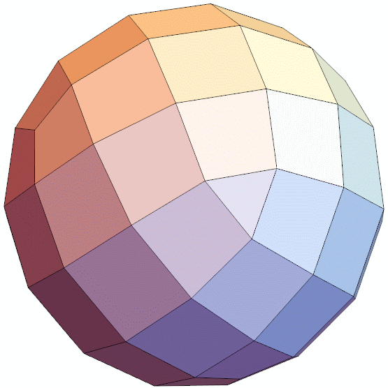
Let's have a look. Doesn't look too much different. Unfortunately, a lot of unit diagonals are gone.
Graphics3D[{Polygon[canonical76[[#]]] & /@ faces}, Boxed -> False, ViewAngle -> Pi/10, ImageSize -> {600, 600}]
Why is that nice? Since this is a self-dual polyhedron, we can combine it with the dual so that all edges intersect and are perpendicular to each other.
Graphics3D[{Polygon[canonical76[[#]]]&/@faces, Polygon[-canonical76[[#]]]&/@faces},Boxed->False,ViewAngle->Pi/10,ImageSize->{600,600}]
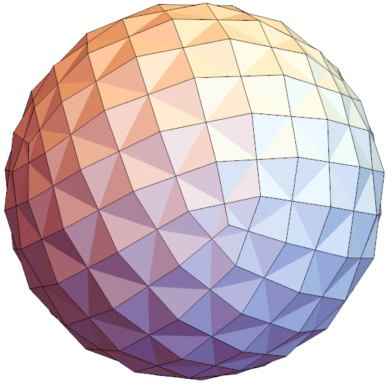
That doesn't happen in my unit diagonal and volume-optimized version, many diagonals are skew and don't intersect.
Graphics3D[{Polygon[verts[[#]]]&/@faces, Polygon[-canonical76[[#]]]&/@faces},Boxed->False,ViewAngle->Pi/10,ImageSize->{600,600}]
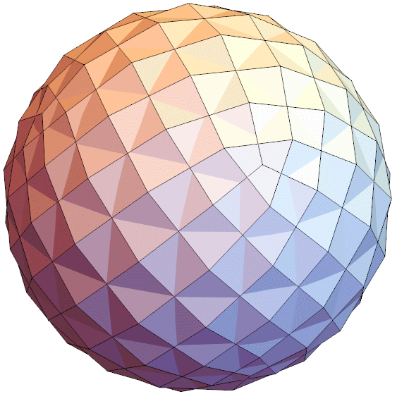
In short, for a formal proof that this is a solid of constant width, it fails. The currently given solution is off by an amount that wouldn't be detectable if it were 3D printed, but it's still not perfect. However, it's very likely fixable by giving up the volume optimization, and instead going for a canonicalization biased optimization, while still maintaining all 150 unit diagonals. That's very doable, I just need to figure out how to do it.