Using Bill Simpsons' starting values one can obtain values for all three parameters (along with an estimate of the mean square error).
s = {{10.7000, 0.2973}, {10.7333, 1.6486}, {10.7833, 3.0039}, {10.8167, 3.5144}, {10.8500, 3.8395},
{10.9000, 4.1202}, {10.9333, 4.2455}, {10.9667, 4.4361}, {11.0167, 4.5758}, {11.0500, 4.6816},
{11.0833, 4.7129}, {11.1333, 4.8043}, {11.1667, 4.9506}, {11.2000, 5.0406}, {11.2500, 5.0837},
{11.2833, 5.2404}, {11.3167, 5.2456}, {11.3667, 5.3305}, {11.4000, 5.3436}, {11.4333, 5.4154},
{11.4833, 5.4245}, {11.5167, 5.4911}, {11.5500, 5.3488}};
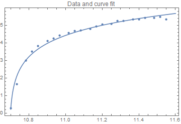
f[t_] = a*Log[b + c*t];
nlm = NonlinearModelFit[s, f[t], {{a, 1.25}, {b, -3100}, {c, 290}}, t]
nlm["BestFitParameters"]
(* {a\[Rule]1.1502828606882431`,b\[Rule]-1631.380481644411`,c -> 152.57998744295452`} *)
nlm["ParameterConfidenceIntervals"]
(* {{1.0474345664791553`,1.253131154897331`},
{-2249.2467635975113`,-1013.5141996913108`},
{94.83889289105193`,210.3210819948571`}} *)
nlm["CorrelationMatrix"]
(* {{1.`,0.9878056648705695`,-0.9878158479618072`},{0.9878056648705695`,1.`,-0.9999998678174467`},
{-0.9878158479618071`,-0.9999998678174467`,1.0000000000000002`}} *)
One can see that the confidence intervals appear wide (at least to me) for the estimates of b and c and the correlations among the parameter estimators are extremely high. Those high correlations cause part of the reason as to why with this model and data, one needs to start close to the final values to obtain convergence.
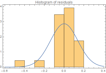
One should also always look at residual diagnostic plots to see if there's anything odd about the fit.
(* Get various quantities from the regression *)
residuals = nlm["FitResiduals"];
predicted = nlm["PredictedResponse"];
residMean = Mean[residuals];
residSD = StandardDeviation[residuals];

(* Data and curve fit *)
Show[{ListPlot[s], Plot[nlm[t], {t, 10.7, 11.6}]}, PlotRange -> All, PlotLabel -> "Data and curve fit", Frame -> True]
(* Histogram of residuals *)
Show[{Histogram[residuals, Automatic, "PDF"],
  Plot[PDF[NormalDistribution[residMean, residSD], x], {x, -0.6, 0.4}]},
  PlotRange -> All, PlotLabel -> "Histogram of residuals", Frame -> True, AxesOrigin -> {-0.6, 0}]
(* Predicted vs. residual *)
ListPlot[Transpose[{predicted, residuals}], PlotLabel -> "Residuals vs. fitted values", Frame -> True]
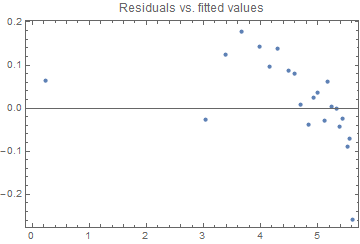
We see that there is a definite lack of fit based on the Residuals vs. fitted values figure. Maybe the theoretical curve needs additional parameters. Maybe there is serial correlation between neighboring measurements. But something you need to ascertain.
Finally a quantile plot is sometimes handy for seeing if the residuals are behaving as assumed:
(* Quantile plot *)
QuantilePlot[residuals, NormalDistribution[residMean, residSD],
 PlotRange -> All, PlotLabel -> "Quantile plot", Frame -> True]
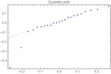
Here we see the first two observations deviate from the (dotted) line associated with a normal distribution. Maybe some transformation of the left and/or right side of the equation might be warranted.


