This may or may not be a good place to drop my armchair math question, since it also involves apparent patterns related to primes.

I recently doodled with prime-generating polynomials of form x^2 + x + n. An approximation of these can be computed for odd values of n up to 200000 and checking values of x for each of them up to 20000 with the following piece of code (note that this code is here for reproducibility, not elegance):

ClearAll[abundances];

abundances = 
  ParallelTable[{a, #} &[
    Divide @@ 
     Sum[With[{n = i^2 + i + a}, {Boole@PrimeQ[n] Log[N@n]/2, 1}], {i,
        20000}]], {a, 1, 200000, 2}];

Beware, this code probably takes an hour or so to run. Smaller values may be a good starting point. Here I use Log as an approximation of the prime density function. It should be good enough for values these polynomials take.

How do the values of n and corresponding relative prime abundances plot out?

ListPlot[abundances, 
 PlotStyle -> Directive[PointSize[Small], Opacity[1/3]], 
 PlotRange -> {{0, 200000}, {1/6, 3 + 1/2}}, 
 Prolog -> {Opacity[1/6], 
   Line@Table[{u, v}, {v, 1/2, 3 + 1/2, 1/2}, {u, 0, 200000, 100000}],
    Line@Table[{u, v}, {u, 0, 200000, 1000}, {v, 0, 10, 1/16}]}]

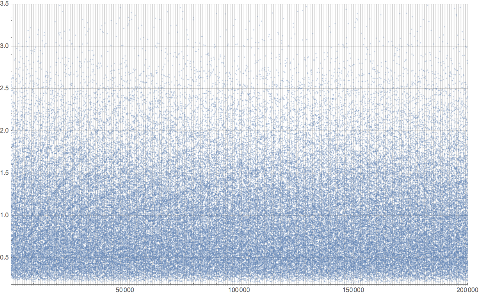
The thing that catches my eye here is that this plot clearly has some structure. What is it? I can't tell.

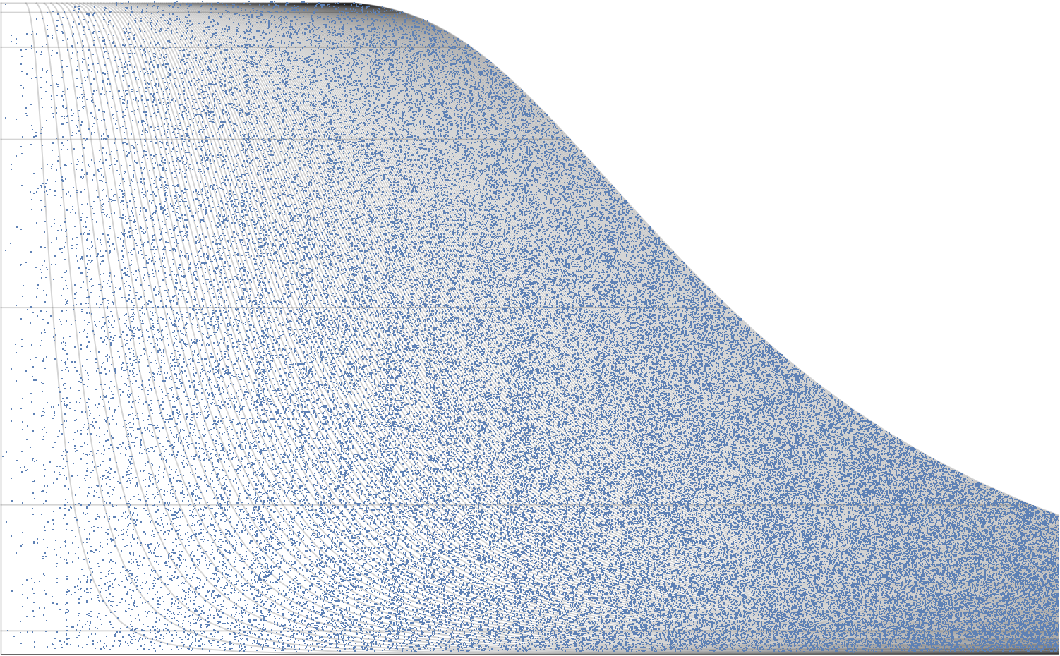
To make these patterns more visible, I project the data in a rather convoluted manner. Note that the grid is the same:

With[{projection = {Sqrt[#1/#2^1.71], 
     CDF[MaxwellDistribution[0.9420730563157451], #2]} &}, 
 ListPlot[projection @@@ abundances, 
  PlotRange -> {{0, Sqrt[abundances[[-1, 1]]/3.5^1.71]}, {0, 1}}, 
  PlotStyle -> Directive[PointSize[Small], Opacity[1]],
  Ticks -> False, 
  Prolog -> {Opacity[1/3], 
    Line@Table[
      projection[u, v], {v, 1/2, 3 + 1/2, 1/2}, {u, 0, 200000, 
       100000}], 
    Line@Table[
      projection[u, v], {u, 0, 200000, 1000}, {v, 1/16, 3 + 1/2, 
       1/16}]}]]

Now those streaks (or patches) are very much visible. Can anyone explain what causes them? Are they actually artefacts of my approximation of prime abundance, or is there something real into it?

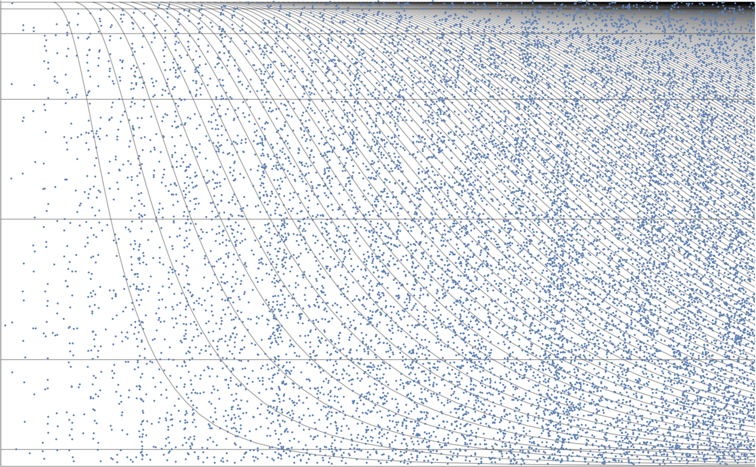
EDIT:

A bit wider plot to show that streaks continue to appear even after the rather narrow projected slice which was shown above:

Here's some code that facilitates exploration of the ideas. The notion is that perhaps Machine Learning can be used to compute the next prime mod 3 from some sequence of preceding primes mod 3. The optional argument digitToCheck extends the idea to see whether one could predict the nth digit of the a prime from the nth digit of its predecessor primes. (all mod 3)

 cm[predecessors_Integer, trainingRange_: {4, 10000}, 
   testingRange_: {10001, 20000}, digitToCheck_: - 1] := 
  Module[{trainingData = 
     Map[Most@# -> Last@# &, 
      Partition[
       Map[IntegerDigits[#, 3][[digitToCheck]] &, 
        Table[Prime[i], {i, trainingRange[[1]], trainingRange[[2]]}]], 
       predecessors + 1, 1]], c, m},

   c = Classify[trainingData];
   m = ClassifierMeasurements[c, 
     Map[Most@# -> Last@# &, 
      Partition[
       Map[IntegerDigits[#, 3][[digitToCheck]] &, 
        Table[Prime[i], {i, testingRange[[1]], testingRange[[2]]}]], 
       predecessors + 1, 1]]];
   Sow[Association["Classifier" -> c, "ClassifierMeasurements" -> m, 
     "Predecessors" -> predecessors, "TrainingRange" -> trainingRange, 
     "TestingRange" -> testingRange]];
   m["Accuracy"]
   ]

And here are some preliminary experiments you can run:

 cm[1, {10000, 19999}, {50000, 
   59999}, -1](* just use immediate predecessor *)

 cm[2, {10000, 19999}, {50000, 59999}, -1](* two predecessors *)

 cm[3, {10000, 19999}, {50000, 59999}, -1](* three predecessors *)

 cm[1, {10000, 19999}, {50000, 
   59999}, -1](* training and testing data far apart *)

 cm[1, {20000, 29999}, {50000, 
   59999}, -1](* different training data far apart *)

 cm[1, {10000, 19999}, {50000, 
   59999}, -2] (* just use immediate predecessor but check whether the \
 second to last digit predicts *)

 cm[2, {10000, 19999}, {50000, 
   59999}, -2](* two predecessors but check whether the second to last \
 digit predicts*)