Message Boards Message Boards

1
|
11661 Views
|
10 Replies
|
7 Total Likes
View groups...
Share
Share this post:

Hypergeometric 2F1 function plotting problem

Posted 11 years ago
I’m attempting to plot a hypergeometric function with complex arguments. I know that this function is defined over all the reals. However, according to Mathematica, the function become indeterminate by x=+20 and x=-20. I’ve attempted to change the workingprecision option of plot to a value of 2000, but the function is still shown to be indeterminate by x=-2500 and x=+2500. Is there a way that I can change this?
q = 3
p = 3
v = 1.1
A = 0.5 + 0.5 I
B = -1 + I
Plot[Re[Exp[-2 I p x]*(Conjugate[A]*Cosh[q - x]^(v + 1)* Hypergeometric2F1[0.5 (v + 1 - I), 0.5 (v + 1 + I), 1/2, -Sinh[q - x]^2] + Conjugate[B]*Cosh[q - x]^(v + 1)*Sinh[q - x]* Hypergeometric2F1[0.5 (v + 1 - I) + 0.5, 0.5 (v + 1 + I) + 0.5, 3/2, -Sinh[q - x]^2])*(A*Cosh[q + x]^(v + 1)* Hypergeometric2F1[0.5 (v + 1 + I), 0.5 (v + 1 - I), 1/2, -Sinh[q + x]^2] + B*Cosh[q + x]^(v + 1)*Sinh[q + x]* Hypergeometric2F1[0.5 (v + 1 + I) + 0.5, 0.5 (v + 1 - I) + 0.5, 3/2, -Sinh[q + x]^2])], {x, -30, 30}]


Thanks.
POSTED BY: John Smith 1
10 Replies
1. Your input for the plot uses machine precision numbers. So, increasing working precision does not really help.

2. More importantly you are plotting a sum of rapidly growing terms which mostly cancel. As a consequence the precision of the output decays rapidly. (If you plot Precion you will see it declines linearly.) When it reaches zero Mathematica will return Indeterminate. My advice, rewrite your function in a way that the individual terms are not manifestly divergent.
Posted 11 years ago
Thanks for your advice. In general, how do I rewrite a function so its terms are not manifestly divergent? Do I use Simplify, FullSimplify, FunctionExpand, or a similar command?
POSTED BY: John Smith 1
You can get the full plot by evaluating the function with sufficiently high precision.

There are two steps in the following approach that worked for me:
  • remove the floating point numbers from the input
  • use WorkingPrecision as an option to Plot:
 q = 3
 p = 3
 v = 11/10
 A = 1/2 + 1/2 I
 B = -1 + I
 Plot[Re[Exp[-2 I p x]*(Conjugate[A]*Cosh[q - x]^(v + 1)*
       Hypergeometric2F1[1/2 (v + 1 - I), 1/2 (v + 1 + I),
        1/2, -Sinh[q - x]^2] +
      Conjugate[B]*Cosh[q - x]^(v + 1)*Sinh[q - x]*
      Hypergeometric2F1[1/2 (v + 1 - I) + 1/2, 1/2 (v + 1 + I) + 1/2,
       3/2, -Sinh[q - x]^2])*(A*Cosh[q + x]^(v + 1)*
      Hypergeometric2F1[1/2 (v + 1 + I), 1/2 (v + 1 - I),
       1/2, -Sinh[q + x]^2] +
     B*Cosh[q + x]^(v + 1)*Sinh[q + x]*
      Hypergeometric2F1[1/2 (v + 1 + I) + 1/2, 1/2 (v + 1 - I) + 1/2,
       3/2, -Sinh[q + x]^2])], {x, -30, 30}, WorkingPrecision -> 100]

POSTED BY: Brett Champion
Looking at it more closely, the problem runs deepers than I originally thought. The loss of precision is not due to a cancelation of terms, but due to Mathematica's evaluation of the 2F1's. This should not normally happen because for Mathematica's Hypergeometric functions "The precision of the output tracks the precision of the input" (according to the documentation).

Why it doesn't do it in this particular case is somewhat of a mystery, as it could easily switch to evaluating the asymptotic expansion for large arguments. (Which is what it does for most other combinations of the parameters.)
Posted 11 years ago
I've modified my approach so I just look at functions of x and worry about q and p later. I think that if I get this sorted out, including q and p will work. I attempted to graph the hypergeometric function between x=-10 and +10 and the asymptotic expansion for the rest of the values. However, even though I used the unit step function, I'm still getting the combined functions to be indeterminate by x=+20 and x=-20. Changing the workingprecision option will allow me to delay the indeterminacy but it still eventually occurs no matter how large workingprecision is. The first image shows just the asmyptotic expansions while the second image shows the asmyptotic expansion combined with the hypergeometric function. (In this case, v=1 but changing the values of v will have little impact on the function being indeterminate or not.)
v = 1
phi[e] = Arg[Gamma[I]*Exp[-I*Log[2]]/(Gamma[0.5*(v + 1) + 0.5 I]*Gamma[0.5*(1 - (v + 1)) + 0.5 I])]
phi[o] = Arg[Gamma[I]*Exp[-I*Log[2]]/(Gamma[0.5*(v + 2) + 0.5 I]*Gamma[1 - 0.5 (v + 1) + 0.5 I])]
r1 = Abs[Gamma[1/2]*Gamma[-I]* Exp[I*Log[2]]/(Gamma[0.5 (v + 1) - 0.5 I]* Gamma[0.5 (1 - (v + 1)) - 0.5 I])]
r2 = Abs[Gamma[3/2]*Gamma[-I]* Exp[I*Log[2]]/(Gamma[0.5 (v + 2) - 0.5 I]* Gamma[1 - 0.5 (v + 1) - 0.5 I])]
u1 = 2*r1*Cos[Abs[x] + phi[e]]
u2 = 2*r2*Cos[Abs[x] + phi[o]]
Plot[{Re[(A*u1 - B*u2)* UnitStep[-10 - x] + (A*Cosh[x]^(v + 1)* Hypergeometric2F1[(1/2) (v + 1 + I), (1/2) (v + 1 - I), 1/2, -Sinh[x]^2] + B*Cosh[x]^(v + 1)*Sinh[x]* Hypergeometric2F1[(1/2) (v + 1 + I) + (1/ 2), (1/2) (v + 1 - I) + (1/2), 3/2, -Sinh[x]^2])*(UnitStep[x + 10] - UnitStep[x - 10]) + (A*u1 + B*u2)*UnitStep[x - 10]]}, {x, -40, 40}]


Any ideas?

Thanks.
POSTED BY: John Smith 1
You cannot use PDF as images - this is why the upload failed. Please convert to JPG or PNG or GIF.
POSTED BY: Vitaliy Kaurov
Your most recent example contains the undefined symbols u1 and u2.  This prevents Plot from plotting anything outside of the -10 to 10 range.  Since your image also did not get posted, it is difficult to say what is happening.

I did put in some random values for u1 and u2, and everything seemed to be working well as long as I made sure that all my inputs were exact numbers and made the WorkingPrecision reasonably high.
POSTED BY: Karl Isensee
Posted 11 years ago
Thanks for noticing that I forgot to define u1 and u2. . I've now editted my question to include u1 and u2.
POSTED BY: John Smith 1
As Brett indicated, solving numerical problems like this is generally a two step process.  You must remove all floating point numbers from your input, and then use the WorkingPrecision option.  In your most recent example, your input includes floating point numbers, so simply increating the WorkingPrecision is not going to suffice.  Please see the following for a brief discussion on exact vs approximate (or floating point) numbers:

http://reference.wolfram.com/mathematica/tutorial/ExactAndApproximateResults.html

Essentially, your input should not include any decimal points - fractions only.

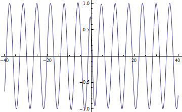
When I made these corrections, I got an acceptable plot:
 v = 1;
 phi[e] = Arg[
 Gamma[i]*
 Exp[-I*Log[2]]/(Gamma[1/2*(v + 1) + 1/2 I]*
 Gamma[1/2*(1 - (v + 1)) + 1/2 I])];
 phi[o] = Arg[
 Gamma[i]*
 Exp[-I*Log[2]]/(Gamma[1/2*(v + 2) + 1/2 I]*
 Gamma[1 - 1/2 (v + 1) + 1/2 I])];
r1 = Abs[Gamma[1/2]*Gamma[-I]*
Exp[I*Log[2]]/(Gamma[1/2 (v + 1) - 1/2 I]*
Gamma[1/2 (1 - (v + 1)) - 1/2 I])];
r2 = Abs[Gamma[3/2]*Gamma[-I]*
Exp[I*Log[2]]/(Gamma[1/2 (v + 2) - 1/2 I]*
Gamma[1 - 1/2 (v + 1) - 1/2 I])];
u1 = 2*r1*Cos[Abs[x] + phi[e]];
u2 = 2*r2*Cos[Abs[x] + phi[o]];
q = 3;
p = 3;
v = 11/10;
A = 1/2 + 1/2 I;
B = -1 + I;
Plot[{Re[(A*u1 - B*u2)*
UnitStep[-10 -
x] + (A*Cosh[x]^(v + 1)*
Hypergeometric2F1[(1/2) (v + 1 + I), (1/2) (v + 1 - I),
1/2, -Sinh[x]^2] +
B*Cosh[x]^(v + 1)*Sinh[x]*
Hypergeometric2F1[(1/2) (v + 1 + I) + (1/
2), (1/2) (v + 1 - I) + (1/2),
3/2, -Sinh[x]^2])*(UnitStep[x + 10] -
UnitStep[x - 10]) + (A*u1 + B*u2)*UnitStep[x - 10]]}, {x, -40,
40}, WorkingPrecision -> 40]
POSTED BY: Karl Isensee
John you tried to upload images in .PDF format - this is why they are not displayed. Could you please re-upload them in .PNG or .JPG or .GIF formats - as you did in your original post?
POSTED BY: Moderation Team
Reply to this discussion
Community posts can be styled and formatted using the Markdown syntax.
Reply Preview
Attachments
Remove
or Discard

Group Abstract Group Abstract