Some days ago, after the most deadly mass shooting in recent US history in Orlando, a colleague and friend of mine Professor Celso Grebogi sent me an article that compared the availability of gun shops to coffee shops in the US. It presents striking representations that are easy to reproduce in the Wolfram Language as we will see below. I also wanted to go a bit beyond the comparison of coffee and gun shops, and used data of a couple of years of mass shootings in the US for a comparison. The article links to a website of the ATF (Bureau of Alcohol, Tobacco, Firearms and Explosives) that offers data on all (official) gun shops in the US. I downloaded the" latest complete listing" and then imported the file:
data = Import["/Users/thiel/Desktop/0516-ffl-list.txt", "TSV"];
Alternatively, you can import directly from the website:
data=Import["https://www.atf.gov/firearms/docs/0516-ffl-listtxt/download"];
The data contains
Length[data]
79447 entries, the first two of which are headers. For each entry the dataset contains the following information:
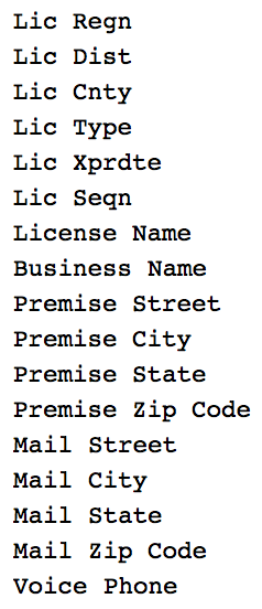
We are only interested in the establishments which have licence types 1 and 2, which leaves us with:
Select[data, (#[[4]] == 1 \[Or] #[[4]] == 2) &] // Length
64483 entries. We will not make heavy use of the Interpreter function. I could have used SemanticImport, but in spite of the relatively slow evaluation of the following line, it is quite straight forward to understand:
citiesguns = (Interpreter["City"][#] & /@
DeleteDuplicates[StringJoin[#[[1]], ", ", #[[2]]] & /@ Select[data, (#[[4]] == 1 \[Or] #[[4]] == 2) &][[1 ;;, {10, 11}]]]);
You can safely ignore potential warnings. Not all entries were properly resolved:
citiesguns // Length
gives 16390, whereas
Select[citiesguns, Head[#] == Entity &] // Length
only gives 13313 entries. I will only use the correct entries and save them into a file:
Export["~/Desktop/citiesgunsok.csv", Select[citiesguns, (Head[#] == Entity) &]];
citiesguns = ToExpression /@ Flatten[Import["~/Desktop/citiesgunsok.csv", "TSV"], 1];
Let's plot that:
styling = {GeoBackground ->GeoStyling["StreetMapNoLabels",GeoStylingImageFunction -> (ImageAdjust@
ColorNegate@ColorConvert[#1, "Grayscale"] &)],GeoScaleBar -> Placed[{"Metric", "Imperial"}, {Right, Bottom}],GeoRangePadding -> Full,ImageSize -> Large};
GeoListPlot[Select[citiesguns, Head[#] == Entity &][[1 ;;]], GeoRange -> Entity["Country", "UnitedStates"], ImageSize -> Full, PlotMarkers -> Point, PlotStyle -> PointSize[0.002], styling]
where my thanks as always goes to @Bernat Espigule for the styling.
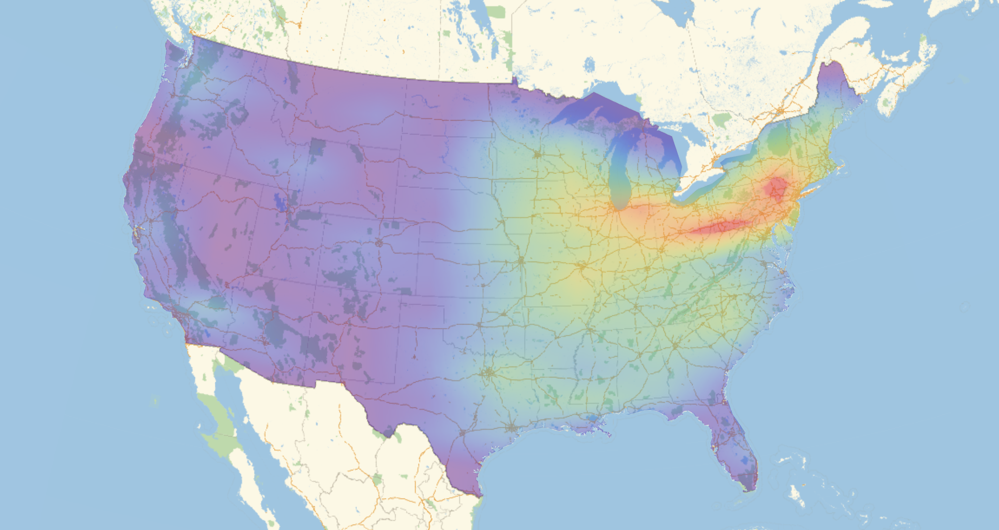
So these are all the gun dealers. We can now also create a histogram:
coords = EntityValue[citiesguns, "Coordinates"];
shopDensityDistribution = SmoothKernelDistribution[RandomChoice[DeleteCases[coords, {"", ""}], 2000], "SheatherJones"];
cplot = ContourPlot[PDF[shopDensityDistribution, {y, x}], Evaluate@
Flatten[{x, {#[[1, 1, 2]], #[[2, 1, 2]]} &@GeoBoundingBox[Entity["Country", "UnitedStates"]]}],
Evaluate@Flatten[{y, {#[[1, 1, 1]], #[[2, 1, 1]]} &@GeoBoundingBox[Entity["Country", "UnitedStates"]]}],
ColorFunction -> "Rainbow", Frame -> False, PlotRange -> All, Contours -> 405, MaxRecursion -> 2,
ColorFunction -> ColorData["TemperatureMap"], PlotRangePadding -> 0, ContourStyle -> None, ImageSize -> Full];
GeoGraphics[{Opacity[0.5], GeoStyling[{"GeoImage", cplot}], Polygon[Entity["Country", "UnitedStates"]]},
 GeoRange -> Entity["Country", "UnitedStates"], ImageSize -> Full]
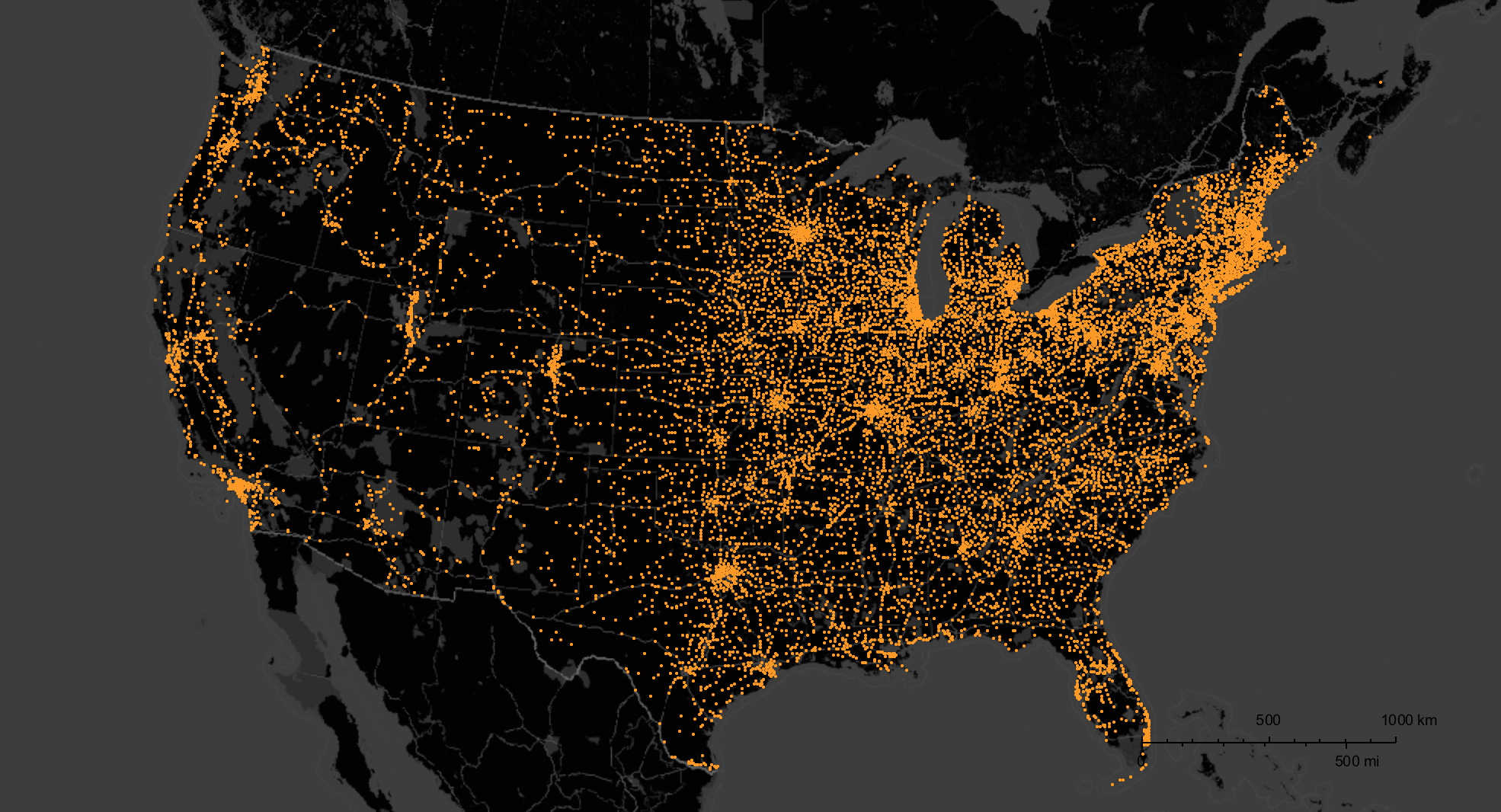
This we can then combine with our gun dealer plot:
GeoGraphics[{Opacity[0.6], GeoStyling[{"GeoImage", cplot}], Polygon[Entity["Country", "UnitedStates"]], Yellow, Opacity[0.6],
PointSize[0.002], Point[Select[Reverse /@ coords, 25.1246 < #[[2]] < 49.3845 && -124.733 < #[[1]] < -66.9498 &]]},
GeoRange -> Entity["Country", "UnitedStates"], ImageSize -> Full, styling]
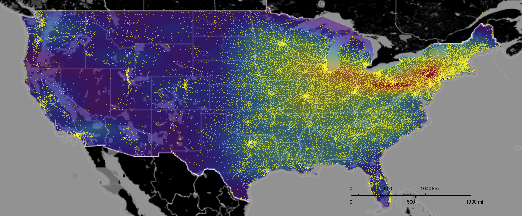
This image does not tell the entire story because it only really plots the cities with shops. In many cities there are multiple dealers, of course. We will later produce a plot which represents that. But before we go there we will use the power of the Wolfram Language to combine different data sets from many different sources. There have been several posts for example by @Jofre Espigule for the year 2016 and by @Dan Lou before that. I will here use Dan Lou's data updated for 2016 including the Orlando shooting and the mass shootings that have happened in the couple of days between Orlando and now. You can get all files from this website.
shootings2016 = Import["~/Desktop/2016CURRENT.csv"];
shootings2015 = Import["~/Desktop/2015CURRENT.csv"];
shootings2014 = Import["~/Desktop/2014MASTER.csv"];
shootings2013 = Import["~/Desktop/2013MASTER.csv"];
shootings = Join[shootings2013[[2 ;;]], shootings2014[[2 ;;]], shootings2015[[2 ;;]], shootings2016[[2 ;;]]];
We now need to find out where the shootings happened; we will do this in two steps to save time:
shootingcoords = CityData[Entity["City", {#[[3]], #[[2]], "UnitedStates"}], "Coordinates"] & /@ shootings;
shootingcoordscorr = (If[Head[#[[1]]] == Missing, (Interpreter["City"][StringJoin[Riffle[#[[2, {3, 2}]], ", "]]])["Coordinates"], , #[[1]]]) & /@
Transpose[{shootingcoords, shootings}];
Not very clean code but it does the trick. There are 1002 shootings for the last years (nearly one shooting every day!) in the database
Select[shootingcoordscorr, Head[#] == List &] // Length
922 of which we can use. We next create a list of coordinates and info on how many people were killed and injured.
coordskilled = Flatten /@ Transpose[{shootingcoordscorr, shootings[[;; , {6, 7}]]}];
When we plot this
GeoGraphics[GeoDisk[#[[{1, 2}]], Quantity[10. #[[-2]], "Kilometers"]] & /@ (Select[coordskilled, Length[#] == 4 \[And] NumberQ[#[[-2]]] &]),
GeoRange -> Entity["Country", "UnitedStates"]]
we obtain the following tragic result:
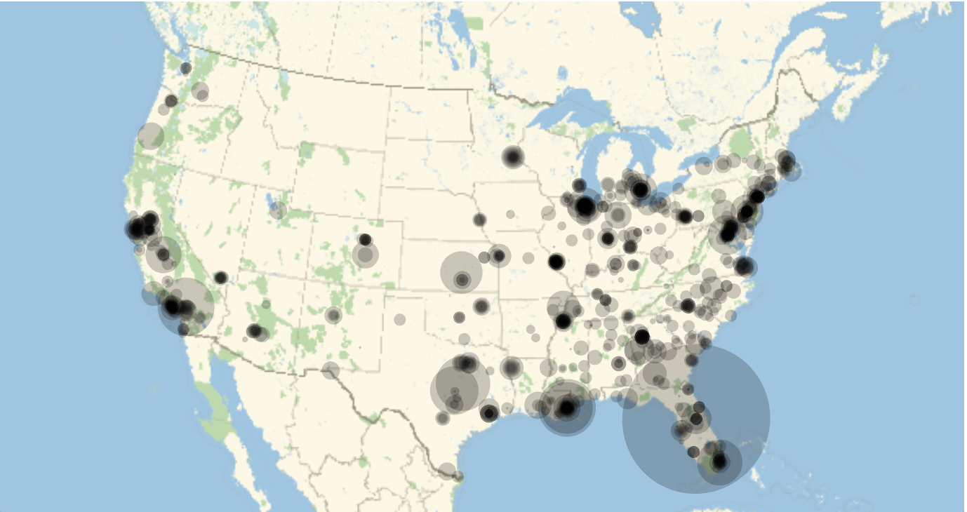
The largest circle in Florida corresponds to the Orlando shooting. Note that the radius of the discs is proportional to the people killed - it might have been better to make the area proportional to the people killed. It is obvious that there is a correlation between shop density and locations of shootings, but that could be because of the very heterogeneous population density in the United States. The curated data in the Wolfram Language can help us to build a graphic on population and population density for the US.
subdivisions = #["Subdivisions"] & /@ Entity["Country", "UnitedStates"]["AdministrativeDivisions"];
countyData = {#, #["Population"], #[EntityProperty["AdministrativeDivision", "PerCapitaIncome"]], #[EntityProperty["AdministrativeDivision","BorderingCounties"]]} & /@ Flatten[subdivisions];
GeoRegionValuePlot[Rule @@@ Transpose[{countyData[[All, 1]], countyData[[All, 2]]}], ImageSize -> 1000, ColorFunction -> (ColorData["Rainbow"][#^.2] &), GeoRange -> Entity["Country", "UnitedStates"]]
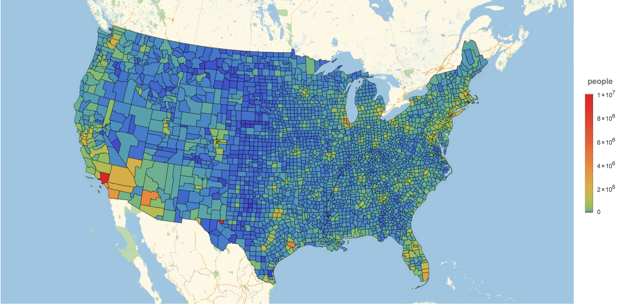
which shows the absolute number of people living in the counties and
countypopdensityData = {#, #["Population"], #["PopulationDensity"]} & /@ Flatten[subdivisions];
GeoRegionValuePlot[Rule @@@ Transpose[{countyData[[All, 1]], countypopdensityData[[All, 3]]}], ImageSize -> 1000,
ColorFunction -> (ColorData["Rainbow"][#^.2] &), GeoRange -> Entity["Country", "UnitedStates"]]
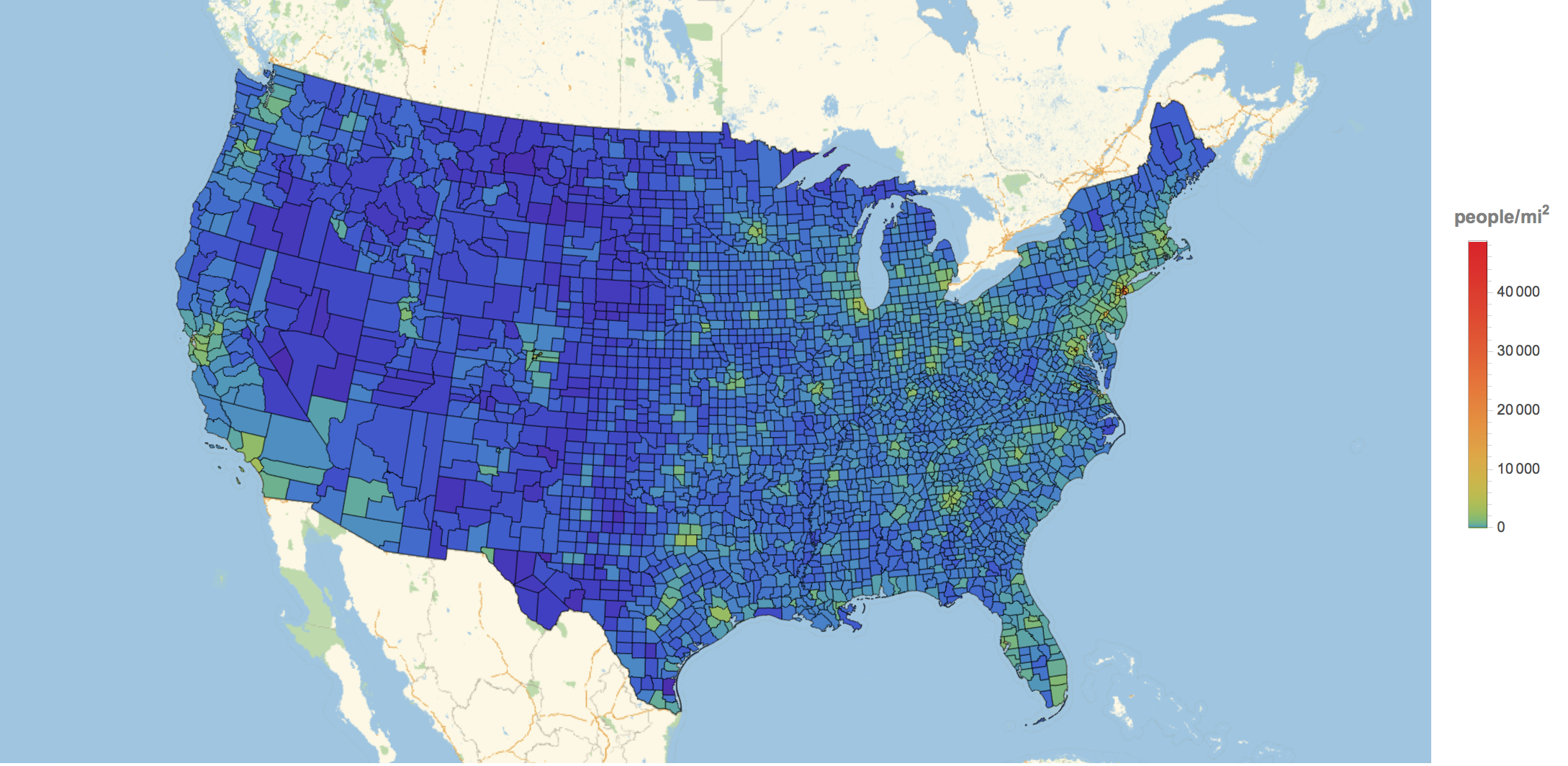
for the population density. So there is an obvious correlation between many people and many shootings. The question is: Can we find anything beyond that in the data?
Let's first try to get some insight into the number of gun dealers in the United States:
rules = (# -> Interpreter["City"][#] & /@ DeleteDuplicates[StringJoin[#[[1]], ", ", #[[2]]] & /@
Select[data, (#[[4]] == 1 \[Or] #[[4]] == 2) &][[1 ;;, {10, 11}]]]);
tallyshops = Reverse@SortBy[Tally[Select[rules[[1 ;;, 2]], Head[#] == Entity &]],Last];
dispatchrules = Dispatch[rules];
citiesmultiplestores = (StringJoin[#[[1]], ", ", #[[2]]] & /@ Select[data, (#[[4]] == 1 \[Or] #[[4]] == 2) &][[All, {10, 11}]]) /. dispatch rules;
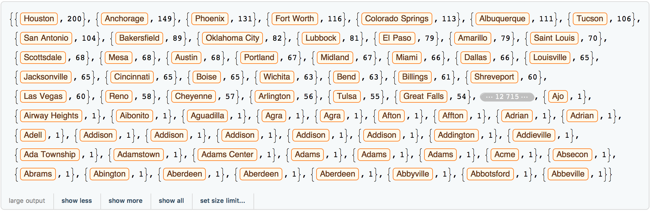
which gives something like:
Reverse[SortBy[Tally[Select[citiesmultiplestores, Head[#] == Entity &]], Last]]
We now calculate some additional lists with data:
citiesshootings = Select[{Entity["City", StringDelete[#, " "] & /@ {#[[3]], #[[2]], "UnitedStates"}], #[[6]]} & /@ shootings, Head[#[[1]]] == Entity &];
dispatchrules2 = Rule @@@ Reverse[SortBy[Tally[Select[citiesmultiplestores, Head[#] == Entity &]], Last]];
totaldeathspercity = {#[[1, 1]], Total[#[[All, 2]]]} & /@ GatherBy[citiesshootings, First];
gunshopsvsdeatsh = Cases[totaldeathspercity /. dispatchrules2, {_Integer, _Integer}];
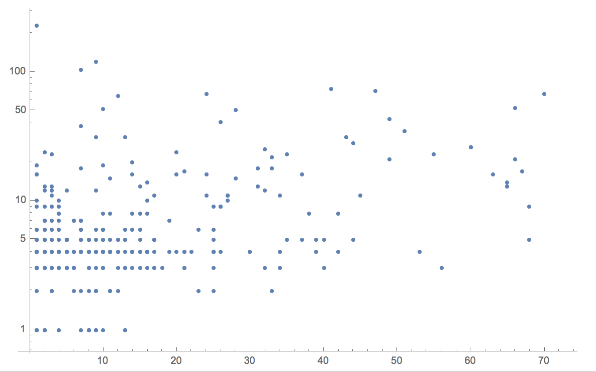
We see for example that there is no convincing correlation between gun shops and deaths:
ListLogPlot[gunshopsvsdeatsh]
We can now rank the cities with respect to the number of gun dealerships:
ListLogLogPlot[Reverse[SortBy[Tally[Select[citiesmultiplestores, Head[#] == Entity &]], Last]][[;; , 2]], PlotRange -> All, Filling -> Bottom,
 AxesLabel -> {"Rank", "Stores"}, LabelStyle -> Directive[Bold, Medium]]
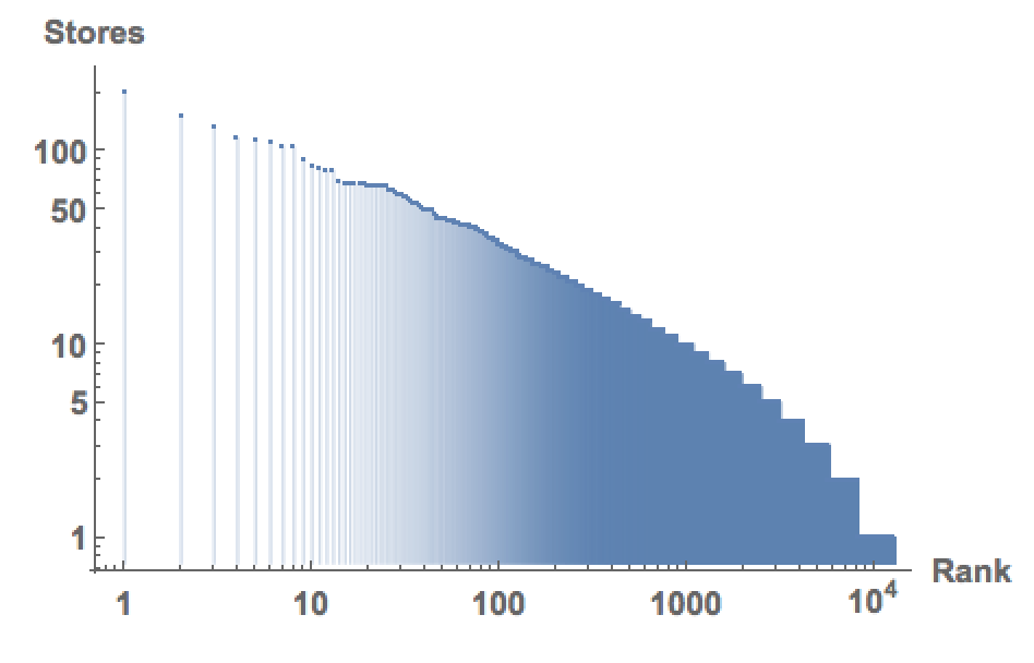
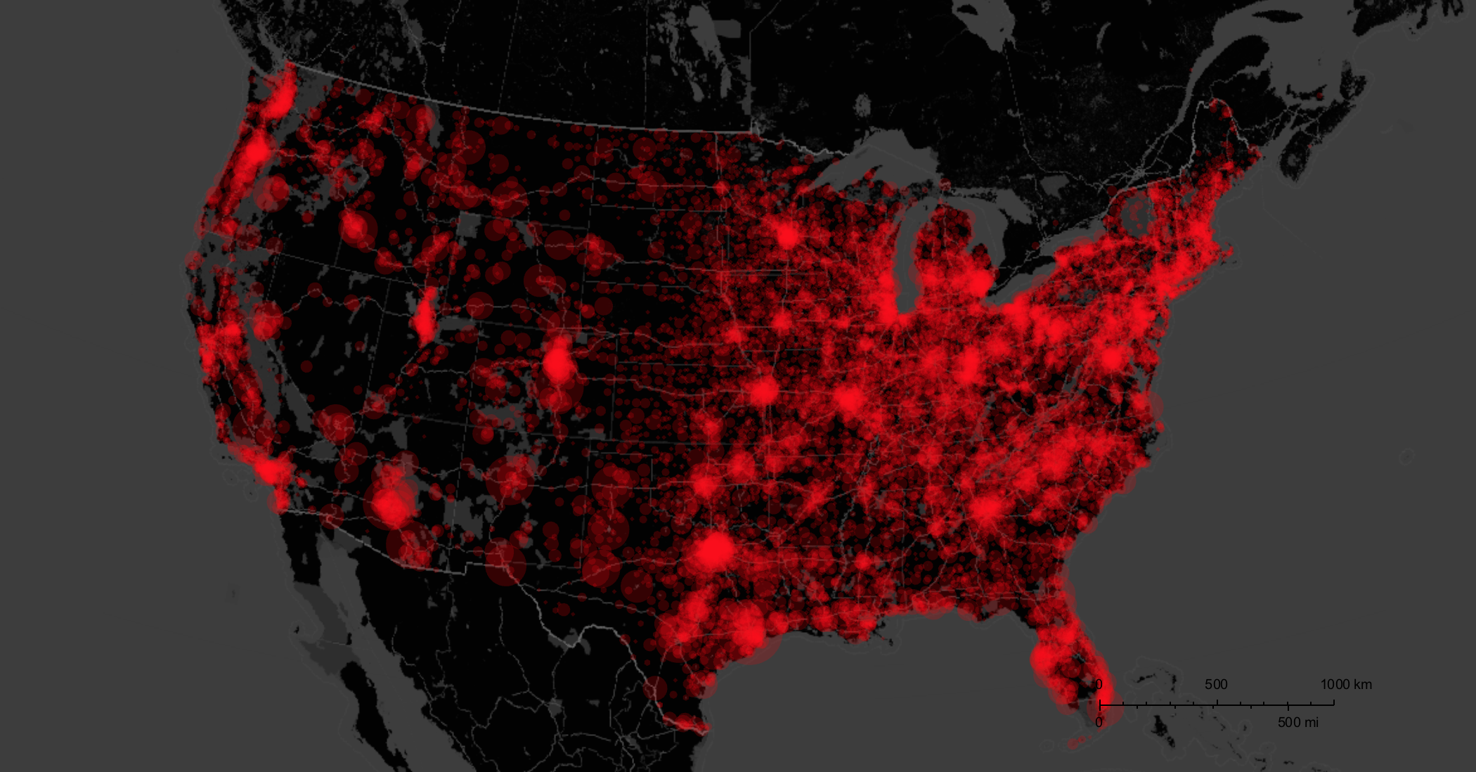
We see that some cities have massive numbers of stores. The following representation tries to show that:
shopsincity = Reverse[SortBy[Tally[Select[citiesmultiplestores, Head[#] == Entity &]], Last]];
GeoGraphics[{Red, GeoDisk[#[[1]], Quantity[10. Sqrt[#[[2]]], "Kilometers"]] & /@ shopsincity}, GeoRange -> Entity["Country", "UnitedStates"],
ImageSize -> Full, styling]
In what is about to be discussed we will need the following two auxiliary lists:
gunshopspercity = Rule @@@ shopsincity[[;; , {1, 2}]];
citieskilled = citiesshootings[[All, 1]];
We now ask the following question: How many gun shops are close to the location of the shootings. We choose neighbouring cities at a distance less than 40km.
Dynamic[ProgressIndicator[1. k/Length[coordskilled]]]

Monitor[shopsclose =
Table[If[Length[coordskilled[[k]]] < 4, "NA", Total[Select[Select[GeoNearest["City",
GeoPosition[coordskilled[[k, {1, 2}]]], 5], GeoDistance[GeoPosition[coordskilled[[k, {1, 2}]]], #] < Quantity[40, "Kilometers"] &] /. gunshopspercity,
NumberQ[#] &]]], {k, 1, Length[coordskilled]}], k]
Some of the data took a while to generate so we better save it:
alldata = Flatten /@ Transpose[{citieskilled[[All, 1]], coordskilled, shopsclose}];
Export["~/Desktop/allshootingdata.csv", alldata];
We can now plot a histogram of how many shops were close to the shootings.
Histogram[{DeleteCases[shopsclose, "NA"]}, 120, "PDF", AxesLabel -> {"close shops", "prob."}, LabelStyle -> Directive[Bold, Medium]]
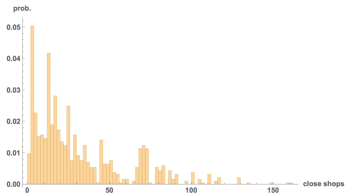
The problem is that this does not tell us much. Let's see whether there is a higher gun availability close to the locations of the shootings than on average. We will proceed as follows: we will estimate the gun dealer availability for an "average American citizen". This estimate won't be perfect, but hopefully suffices for our purpose. Our algorithm is as follows: we will generate a list of all cities that are in the curated database of Wolfram. Then we will use their populations to "draw a random American citizen" - we obviously ignore some parts of the population here.
Here are the cities and their populations:
citiespopulationUS = {#, CityData[#, "Population"]} & /@ CityData[{All, "UnitedStates"}];
We then "draw" 1002 random citizens (actually their cities) from this list according to the respective population sizes:
randomcities = RandomChoice[(QuantityMagnitude[citiespopulationUS[[;; , 2]]] /. {QuantityMagnitude[Missing["NotAvailable"]] -> 0.} ) -> citiespopulationUS[[;; , 1]], 1002];
We next calculate how many gun dealerships there are close to these imaginary people:
Monitor[shopscloserandom = Table[Total[Select[Select[GeoNearest["City", randomcities[[k]], 5],
GeoDistance[randomcities[[k]], #] < Quantity[40, "Kilometers"] &] /. gunshopspercity, NumberQ[#] &]], {k, 1, Length[coordskilled]}], k]
So this is the average number of gun dealerships close to shooting locations:
Mean[DeleteCases[shopsclose, "NA"]] // N
which gives 35.7354; and this is the average number for an "average citizen":
Mean[shopscloserandom] // N
which gives 24.4112. So there appear to be many fewer shops close to the average person. We can plot the histograms:
Histogram[{shopscloserandom, DeleteCases[shopsclose, "NA"]}, 120, "PDF",
AxesLabel -> {"close shops", "prob."}, LabelStyle -> Directive[Bold, Medium]]
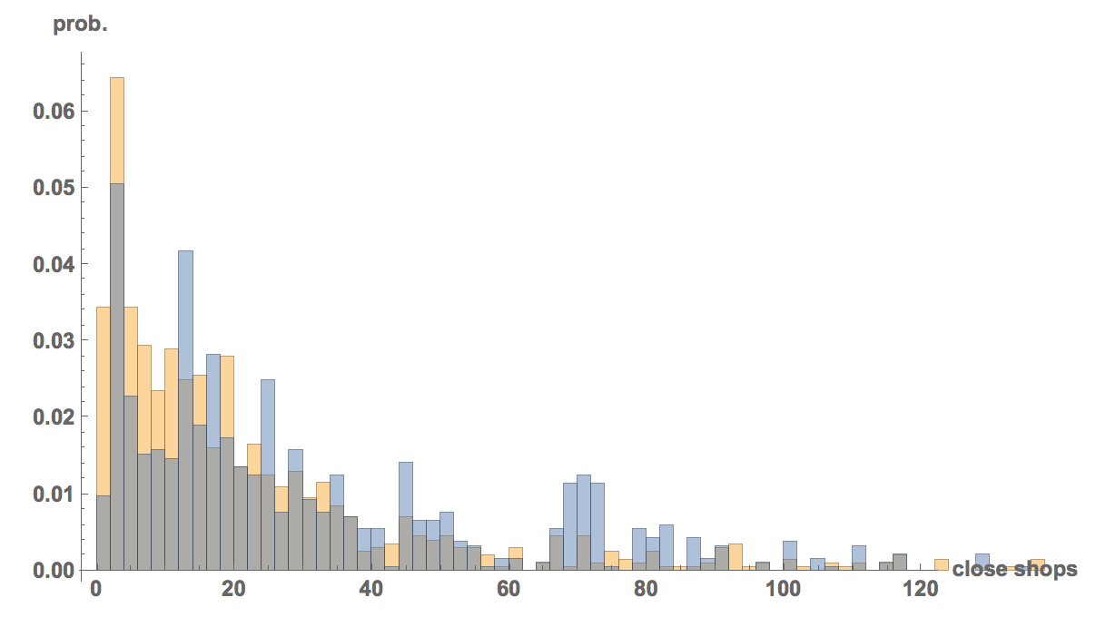
where the orange bars are for our average citizen (control) and the blue ones for the shooting locations. It is relatively obvious that this is statistically significant.
LocationTest[{shopscloserandom, DeleteCases[shopsclose, "NA"]}, Automatic, "TestConclusion"]
which evaluates to:

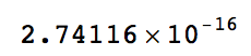
There is, in fact, a very small p-value
LocationTest[{shopscloserandom, DeleteCases[shopsclose, "NA"]}]
There are some pitfalls here, such as that we only look at correlation, which - as we know- does not imply causality. There are many potential confounding factors. It could be that shootings and larger number of gun dealerships are consequences of some common cause such as gang crime etc. Also, some of the smaller cities have not been recognised by Interpreter. We also have ignored the fact that there are often non-fatal injuries:
Histogram[{shootings[[All, 5]], shootings[[All, 6]]}, PlotRange -> {{0, 16}, All}, PlotTheme -> "Detailed"]
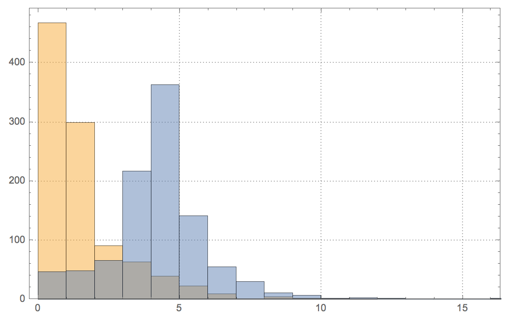
where orange is for deaths and blue for injured. Having said all of this the data suggests a strong correlation between dealerships and shootings.
Also note that the code is not quite clean and optimised. I recalculate many things lots of times and basically post code that I just wrote down without any attempt at optimising it. The CPU time for the entire code is nearly half a day, but could be more on slower machines.
I am planning to run a GLM on this data and see what else we can learn from it.
Cheers,
Marco
PS: @Vitaliy Kaurov, I know that the code is quite inefficient. There is much more WL curated data that could be used. At the Wolfram Technology Tour Europe I have heard some really exciting stuff about future machine learning in Mathematica, which might offer great potential for this type of analysis.


