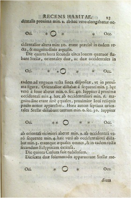
Awhile back, Stephen Wolfram suggested that I try to re-create, using modern calculations instead of observations, Galileo's observations of Jupiter's 4 largest moons. I thought I'd share the results here for fun, especially since its nice of have something about Jupiter given the arrival of the Juno spacecraft at Jupiter this past weekend. These moons are also known today as the Galilean Satellites. At the time, the prevailing view of the cosmos was that Earth was the center of the universe and everything moved around it. So, it came as a surprise when Galileo observed Jupiter through his primitive telescope that Jupiter has 4 "stars" that appeared to be orbiting it. In his diagrams, Jupiter was represented as a simple circle, and the new satellites as star-like figures.

Using Astronomical Algorithms, by Jean Meeus, as a source, I used the low accuracy method (since we just need the results to look okay to the eye) to compute the positions of Jupiter's 4 big moons in 2D. Higher accuracy methods are also provided in the source, but those are used for things like transits, eclipses, etc. and is more than what is needed here.
JovianMoonCoordinates[jd_] :=
 Module[{A, B, d, DE, Delta, DS, du1, du2, du3, du4, G, H, J, KK,
   lambda, M, NN, psi, r, R, r1, r2, r3, r4, u1, u2, u3, u4, V, w1,
   w2}, d = jd - 2451545;
  V = 3.0148817498 + 0.000019475780 d;
  M = 6.2400582213 + 0.017201970 d;
  NN = 0.349414916249264 + 0.0014501120450072 d +
    0.00574213323906134 Sin[V];
  J = 1.15392443495605 + 0.0157519089131849 d -
    0.005742133239061344 Sin[V];
  A = 0.033423055175691 Sin[M] + 0.00034906585039886 Sin[2 M];
  B = 0.096953039948 Sin[NN] + 0.0029321531433504 Sin[2 NN];
  KK = J + A - B;
  R = 1.00014 - .01671 Cos[M] - .00014 Cos[2 M];
  r = 5.20872 - .25208 Cos[NN] - .00611 Cos[2 NN];
  Delta = Sqrt[r^2 + R^2 - 2 r R Cos[KK]];
  psi = ArcSin[R/Delta Sin[KK]];
  w1 = 3.68229565585763 + 15.3207952882387 d -
    0.088559510336640 Delta + psi - B;
  w2 = 3.26777995850898 + 15.18762666631161 d -
    0.087789749516252 Delta + psi - B;
  lambda =
   0.599520598060052 + 0.001450211528774608 d +
    0.005742133239061344 Sin[V] + B;
  DS = 0.0544542726622230 Sin[0.7470009198535 + lambda];
  DE = DS -
    0.02268928027592 (r - Delta)/Delta Sin[
      lambda - 1.754055898254301] -
    0.03874630939427 Sin[psi] Cos[lambda + 0.383972435438752];
  u1 = 2.858969742485099 + 3.5501020551357 d -
    0.0205208211279524 Delta + psi - B;
  u2 = 6.25550438524295 + 1.767872509298387 d -
    0.01021891623871900 Delta + psi - B;
  u3 = 0.0997909453120277 + 0.876757737252356 d -
    0.0050679637991465 Delta + psi - B;
  u4 = 3.923660728774436 + 0.3750360006026911 d -
    0.00216783815377278 Delta + psi - B;
  G = 5.780181416754821 + 0.878083559165341 d -
    0.00507562750962625 Delta;
  H = 1.526290430869041 + 0.37645409807322 d -
    0.002176035248978202 Delta;
  du1 = 0.00825540736193317 Sin[2 (u1 - u2)];
  du2 = 0.0185877565337396 Sin[2 (u2 - u3)];
  du3 = 0.002879793265790643 Sin[G];
  du4 = 0.01471312559431219 Sin[H];
  r1 = 5.9057 - .0244 Cos[2 (u1 - u2)];
  r2 = 9.3966 - .0882 Cos[2 (u2 - u3)];
  r3 = 14.9883 - .0216 Cos[G];
  r4 = 26.3627 - .1939 Cos[H];
  u1 += du1;
  u2 += du2;
  u3 += du3;
  u4 += du4;
  MapThread[{# Sin[#2], -# Cos[#2] Sin[DE]} &, {{r1, r2, r3, r4}, {u1,
      u2, u3, u4}}, 1]]
I created a star symbol to represent the moons using the following:
star[{x_, y_}] :=
 Line[{{{-.75/2 + x, -.75/2 + y}, {.75/2 + x, .75/2 + y}}, {{-.75/2 +
      x, .75/2 + y}, {.75/2 + x, -.75/2 + y}}, {{x,
     1/2 + y}, {x, -1/2 + y}}}]
Finally, the pieces are assembled to create an individual "frame" here:
JupiterSatellites[date_] := Module[{jd = JulianDate[date]},
  Graphics[{GrayLevel[.6], {{Black, star[#]}} & /@
     JovianMoonCoordinates[jd]}, ImageSize -> 400,
   PlotRange -> {{-25, 25}, {-1, 1}}, PlotRangePadding -> 3,
   Epilog -> {White, EdgeForm[Black], Thickness[.003],
     Disk[{0, 0}, {1, 1/1.071}]},
   PlotLabel ->
    Block[{$DateStringFormat = {"MonthNameShort", " ", "DayShort",
        " ", "Year", " ", "Hour12Short", ":", "Minute", "AMPM"}},
     DateString[date]]]]
A sequence of frames is easily created with a simple Table command:
frames = Table[
  JupiterSatellites[
   DateObject[{1610, 1, 8, h, 0, 0}, TimeZone -> 1]], {h, 0, 120, 3}];
And you can view this list of frames as a stacked diagram as follows:
Grid[List/@frames, Dividers -> All]

You can also export the frames as an animation to see the positions change in time.
