This can be done by a slightly "hacky" way WITHIN Mathematica. You may find the data info behind the graphics obj by hitting shift+ctrl+E (on mac: use cmd instead of ctrl) after you choose the graphics. Please follow the short example:
plt = StreamPlot[{-1 - x^2 + y, 1 + x - y^2}, {x, -3, 3}, {y, -3, 3}]
Now you should have a plot stored in the variable "plt". Then use the Part function ([[ ]]) to extract the information from the data list, which is plt as well. The actual index may vary depends upon the graphics object you have. In this paticular case, you can see the data for one stream line
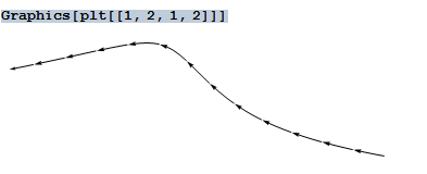
plt[[1, 2, 1, 2]]
You may see the single stream line with graphics command:

To find all such lines, you can use
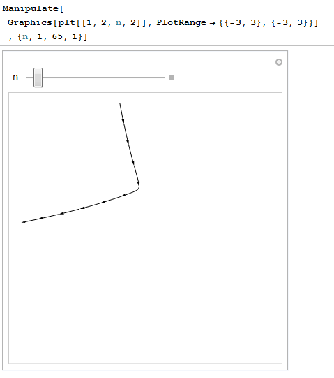
Manipulate to sweep over all possibilities:
Manipulate[
Graphics[plt[[1, 2, n, 2]], PlotRange -> {{-3, 3}, {-3, 3}}]
, {n, 1, 65, 1}]

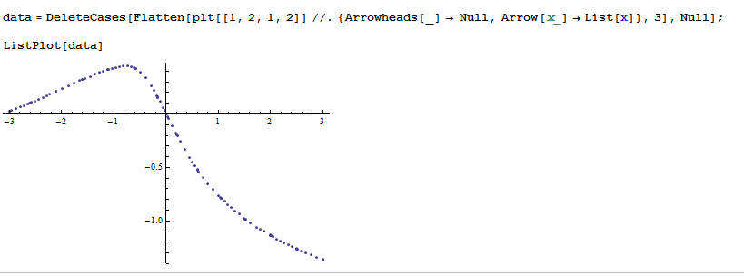
Eventually, you may use the following subroutine to extract the actual data points :
DeleteCases[
Flatten[plt[[1, 2, 1, 2]] //. {Arrowheads[_] -> Null, Arrow[x_] -> List[x]}, 3], Null]
Basically it first
replaces the
Arrowheads objects with Null and Arrow objects with List. It deletes the Null's and converts the list to a proper form with the
Flatten function.
The final result
