Bingo?
I found that for small lists the code Total[Clip[list, {0, [Infinity]}]] is not more the fastest. The fastest is a new piece of code
Plus @@ Clip[list, {0, \[Infinity]}]
but only for lists with small dimensions ( = 20). I have done experiments with the following pieces of code
In[428]:= tList = {
  (* 1*) Total[Clip[list, {0, \[Infinity]}]] // AbsoluteTiming,
  (* 2*) Plus @@ Clip[list, {0, \[Infinity]}] // AbsoluteTiming,
  (* 3*) Total[Select[list, Positive]] // AbsoluteTiming,
  (* 4*) Total[Cases[list, x_ /; x > 0]] // AbsoluteTiming,
  (* 5*) Plus @@ Cases[list, x_ /; x > 0] // AbsoluteTiming,
  (* 6*) Plus @@ Select[list, # > 0 &] // AbsoluteTiming,
  (* 7*) Total[list /. x_ /; x < 0 -> 0] // AbsoluteTiming,
  (* 8*) Total@Map[If[# < 0, 0, #] &, list] // AbsoluteTiming,
  (* 9*) Plus @@ Map[If[# < 0, 0, #] &, list] // AbsoluteTiming,
  (*10*)(s = 0; l = Length[list];
    Do[If[list[[i]] > 0, s += list[[i]], s], {i, l}]; s) //
   AbsoluteTiming,
  (*11*)(s = 0; l = Length[list];
    Table[If[list[[i]] > 0, s += list[[i]], s], {i, l}][[l]]) //
   AbsoluteTiming,
  (*12*)(pcf = Function[x, Piecewise[{{x, x > 0}}, 0], Listable];
    Total[pcf[list]]) // AbsoluteTiming,
  (*13*)(s = 0; l = Length[list];
    For[i = 0, i <= l, i++, If[list[[i]] > 0, s += list[[i]], s]];
    s) // AbsoluteTiming,
  (*14*)(s = 0; i = 1; l = Length[list];
    While[i <= l, If[list[[i]] > 0, s += list[[i]], s]; i++]; s) //
   AbsoluteTiming
  }

Out[428]= {{0.0000371432, 64.4051}, {0.0000244363,
  64.4051}, {0.0000288349, 64.4051}, {0.0000483839,
  64.4051}, {0.0000317672, 64.4051}, {0.0000288349,
  64.4051}, {0.0000562036, 64.4051}, {0.0000498501,
  64.4051}, {0.0000381207, 64.4051}, {0.0000659781,
  64.4051}, {0.0000596246, 64.4051}, {0.0000850384,
  64.4051}, {0.0000762413, 64.4051}, {0.0000772188, 64.4051}}
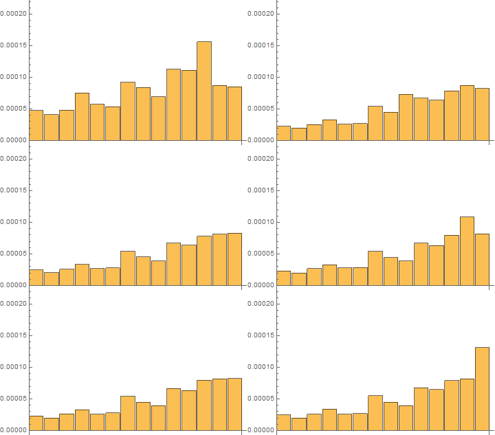
I observed that if the experiments are repeated, the time results are not the same. You can view this fact in the following animation, which includes 120 repetitions of the same summations on the same list.

A question appears: why the times are different if the code and the list remain unchanged?
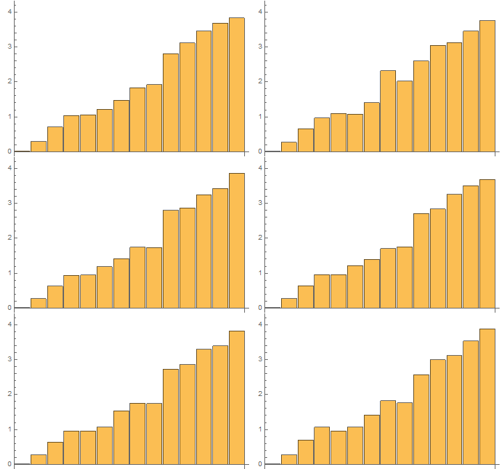
I have done the same experiment on the list with 1 mln elements, but providing repetitions only 32 times. The results may be seen in the following GIF

For the large lists, the time behavior of the pieces of code are more stable.
Nevertheless, one more question appears: what is the worst correct piece of code?
May be the following code a pretender to such denomination?
Total[list //. {a___, b_, c___} /; b < 0 -> {a, 0,
     c}] // AbsoluteTiming
For small lists it works perfect! But for lists with length more than 1000 it requires very long time.