Message Boards Message Boards

1
|
9423 Views
|
1 Reply
|
5 Total Likes
View groups...
Share
Share this post:

Plotting Hermite-Gaussian polynomial for Gaussian beams

Posted 11 years ago
 Hello everyone,  I ve been trying to produce an image comparable to this Wikipedia figure (Twelve Hermite-Gaussian modes). Unfortunately, my plot, although it follows the general pattern as you go ito higher modes, looks rather grainy.  Does anyone know how to produce a fine image like the link above.  or is this the limit of what i can do on Mathematica? The following is my code:
F[n_, m_, x_, y_] = Sqrt[2/(Pi*2^(n + m)*m!*n!)]*HermiteH[m, x]*HermiteH[n, y]*Exp[-x^2]*Exp[-y^2];
DensityPlot[(F[1, 2, x, y]^2), {x, -10, 10}, {y, -10, 10}, PlotRange -> All]
This is the copy of the image from Wikipedia

POSTED BY: seongwoo oh
Welcome to Wolfram Community!

Please note how code, links and images were formatted in your post and follow this format in future.


In your simple case you have to increase PlotPoints option to DensityPlot up to say 50. But... it is always a good idea to search the Wolfram Demonstrations Project for solution of your problem. It also provides code free to download. Here is publication that is relevant to you: 
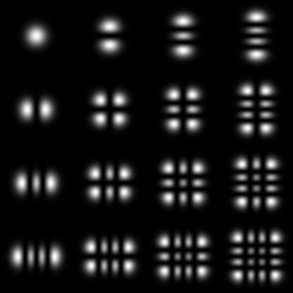
Gaussian Laser Modes.


Adopting code from this Demonstration I could quickly build this image:
 f[n_, x_] := (2/\[Pi])^(1/4) Sqrt[1/(2^n n!)] HermiteH[n, Sqrt[2] x] E^-x^2;
 Intensity[m_, n_, x_, y_] := f[m, x]^2 f[n, y]^2;
 
 GraphicsGrid[ParallelTable[
   DensityPlot[
    Evaluate[Intensity[m, n, x, y]], {x, -2 Sqrt[2],
     2 Sqrt[2]}, {y, -2 Sqrt[2], 2 Sqrt[2]}, Mesh -> None,
    PlotPoints -> 50, ColorFunction -> GrayLevel, PlotRange -> All,
    Frame -> False,
   ImageSize -> 120 {1, 1}, PlotRangePadding -> 0
   ],
  {m, 0, 3},
  {n, 0, 3}], Spacings -> 0, Background -> Black]

POSTED BY: Vitaliy Kaurov
Reply to this discussion
Community posts can be styled and formatted using the Markdown syntax.
Reply Preview
Attachments
Remove
or Discard

Group Abstract Group Abstract