Introduction

I recently came across a post for a computer program that in some fields intends to compete with the Wolfram Language and which has a toolbox for Machine Learning. I wanted to compare the work described with the workflow in Mathematica. The challenge is to classify old Japanese Characters from texts from the so-called Edo period:

Style[StringTake[WikipediaData["Edo period"], 601], 16]

The characters are written in running style and apparently are difficult to read for Japanese speakers today. We will use two approaches of machine learning in the Wolfram Language to tackle this problem.

Historical Background

Before we proceed, let's have a look at the Tokugawa shogunate. I will use code borrow from @Vitaliy Kaurov from his great article on "Computational history: countries that are gone". The following lines compute the historic boundaries of the shogunate:

Monitor[tokugawaPOLY = 
   Table[EntityValue[Entity["HistoricalCountry", "TokugawaShogunate"],
      EntityProperty["HistoricalCountry", 
      "Polygon", {"Date" -> DateObject[{t}]}]], {t, 1600, 1870}];, t]

We then only filter for "changes" in the boundaries:

tokugawaPOLY // Length
tokugawaPOLYcomp = 
  DeleteMissing[
   DeleteDuplicates[Transpose[{Range[1600, 1870], tokugawaPOLY}], 
    Last[#1] == Last[#2] &], 1, 2];
tokugawaPOLYcomp // Length

In the 271 I consider in the first place there are only 4 changes to the boarders, which we can plot like so:

GeoGraphics[{EdgeForm[Red], GeoStyling[Opacity[.1]], #} & /@ 
  tokugawaPOLYcomp[[All, 2]], GeoProjection -> "Mercator", 
 ImageSize -> 800, GeoBackground -> GeoStyling["StreetMap"], 
 GeoRange -> Entity["Country", "Japan"], 
 GeoRangePadding -> Quantity[800, "Kilometers"], GeoZoomLevel -> 6]

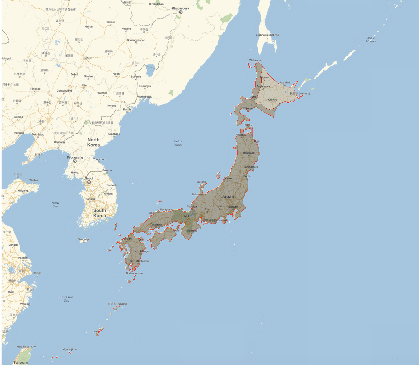
So the boarders were indeed very stable for a long period reflecting the "no more wars" philosophy of the day.

Arts and culture

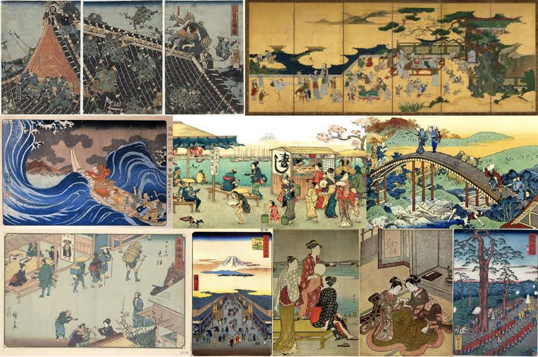
The stability led to a very rich art and literature scene. Here are some images that reflect the style of the time:

ImageCollage["Thumbnail" /. Normal[Normal[WebImageSearch["Edo Period"]]], Method -> "Rows"]

Our dataset

Also literature flourished during this period. Our dataset will be taken from the Center for Open Data in the Humanities. The keen reader might have noticed that the page is in Japanese. Mathematica can translate the page, and so can Google. The dataset is called the "Japanese classic registered glyph data set"; ?????????????.

TextTranslation["?????????????"]

"Japan classics-type datasets". Following the first link (grey box) on the original Japanese page one gets to this page, from the bottom of which (look for a download symbol and the text "(TAR+GZ 24.57 MB)" the dataset can be downloaded. This is the google translation of the reference:

Japanese Classic Statement Character Data Set" (Kokugaku Kenkyu Other Collection / CODH Processing)

which in the original is "???????????????????????CODH??".

The glyphs come from "bamboo letters" from 15 classic texts; the dataset contains more than 20000 glyphs of the 10 most frequent symbols. These letters were annotated by the "National Institute of Letters of Japan" (google). The dataset was also used in a data/machine learning challenge.

After extracting the file to a folder on the desktop I can import the images with:

characterImages = Import["/Users/thiel/Desktop/pmjt_sample_20161116/train_test_file_list.h5", "Data"];

Here is a sample of the glyphs:

Grid[Partition[ImageAdjust[Image[#/256.]] & /@ characterImages[[3, 1 ;; 24]], 6], Frame -> All]

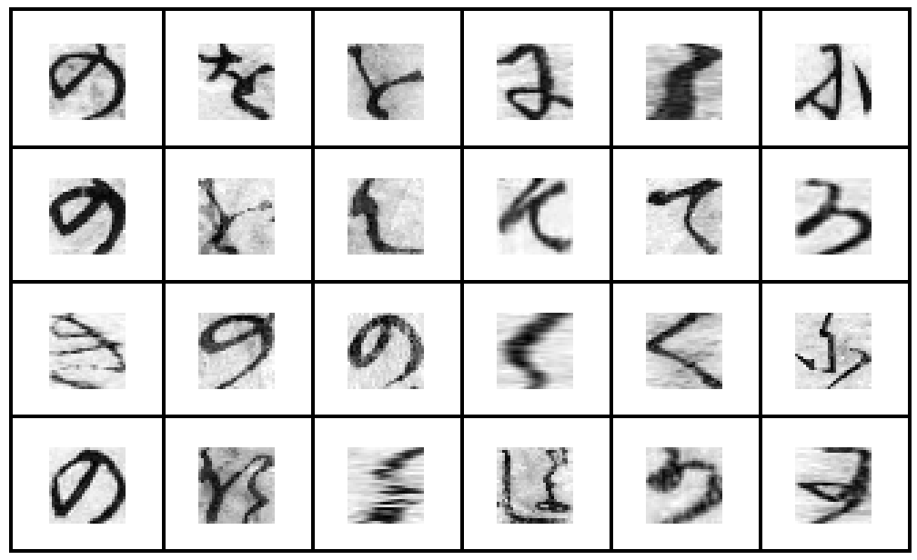
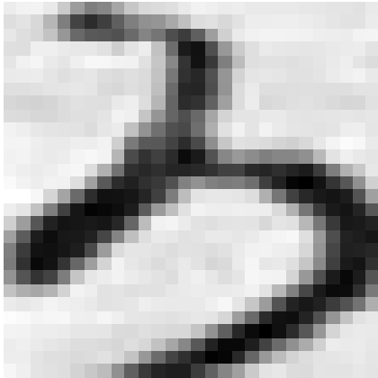
Similar to the MNIST dataset, they consist of 28 times 28 pixels. They give the grey level as integers, which is why I divide by 256. This shows the pixelation of the glyphs:

Image[characterImages[[3, 12]]/256.] // ImageAdjust

The dataset conveniently contains a training and a test set. There are

characterImages[[3]] // Length

19909 glyphs in the training set. All of these are annotated:

Flatten[characterImages[[4]]]

We can convert the training data to images like so:

Monitor[trainingset = Table[ImageAdjust[Image[characterImages[[3, k]]/256.]] -> Flatten[characterImages[[4]]][[k]], {k, 1, 19909}];, k]

The test set contains

characterImages[[1]] // Length

3514 glyphs. The annotation of which are found in

characterImages[[2]] // Flatten // Short

This is how we prepare the test set data for our machine learning:

Monitor[testset = Table[ImageAdjust[Image[characterImages[[1, k]]/256.]] -> Flatten[characterImages[[2]]][[k]], {k, 1, 3514}];, k]

What are the 10 most frequent symbols?

In one of the annotation files we find the character codes of the symbols so that we can map the classification to actual symbols. These are the glyphs we will consider:

Rasterize /@ (Style[
     FromCharacterCode[
      ToExpression["16^^" <> StringJoin[Characters[#]]]], 
     100] & /@ {"3057", "306B", "306E", "3066", "308A", "3092", 
    "304B", "304F", "304D", "3082"})

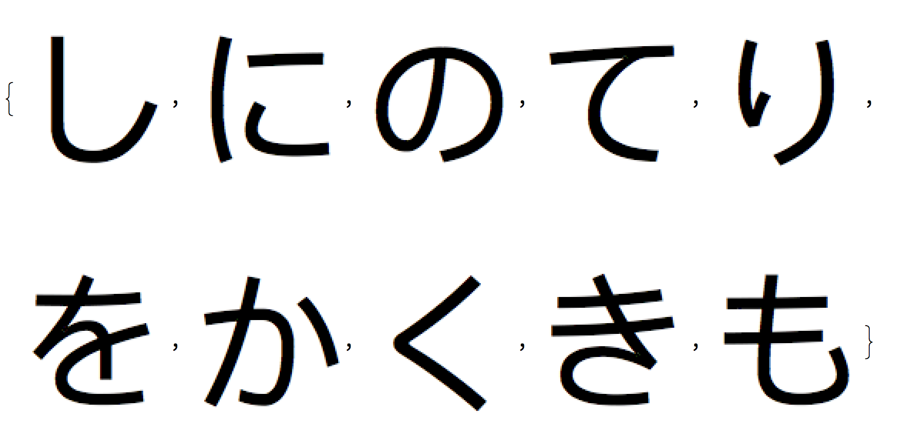
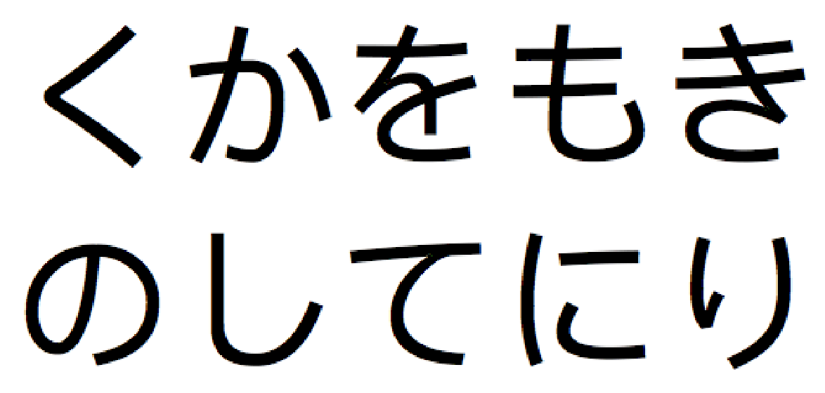
We can also make an image collage of them:

ImageCollage[
 Image /@ (Rasterize /@ (Style[
        FromCharacterCode[
         ToExpression["16^^" <> StringJoin[Characters[#]]]], 
        100] & /@ {"3057", "306B", "306E", "3066", "308A", "3092", 
       "304B", "304F", "304D", "3082"})), Method -> "Rows"]

I though it would be nice if they were in a more calligraphic form. So I tried to used ImageRestyle to try and make them more calligraphic. I think that the attempt was not very successful, but I want to show it anyway.

First I download a couple of calligraphic symbols:

caligraphy = "Thumbnail" /. Normal[Normal[WebImageSearch["japanese calligraphy"]]]

I liked the 5th one, which I will use for the style transfer:

calisymbols = 
 ImageRestyle[#, caligraphy[[5]], 
    PerformanceGoal -> 
     "Quality"] & /@ (Rasterize /@ (Style[
        FromCharacterCode[
         ToExpression["16^^" <> StringJoin[Characters[#]]]], 
        100] & /@ {"3057", "306B", "306E", "3066", "308A", "3092", 
       "304B", "304F", "304D", "3082"}))

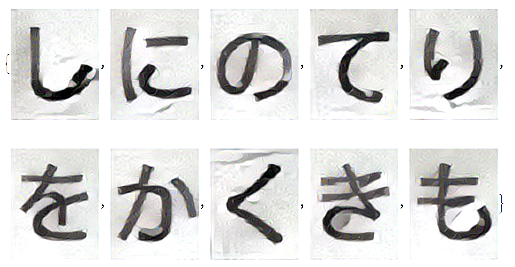
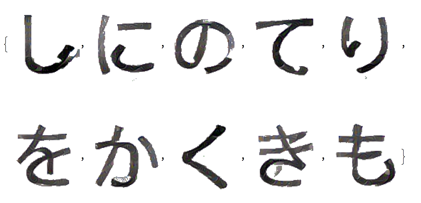
We can also remove the background to get an alternative representation:

Machine Learning (Classify)

Our first approach to classify the glyphs will be via Classify. The classification is very fast (only a couple of seconds on my machine) and quite accurate:

standardcl = Classify[trainingset, ValidationSet -> testset, PerformanceGoal -> "Quality"]

We can first calculate the ClassifierMeasurements

cmstandard = ClassifierMeasurements[standardcl, testset]

and the accuracy:

cmstandard["Accuracy"]

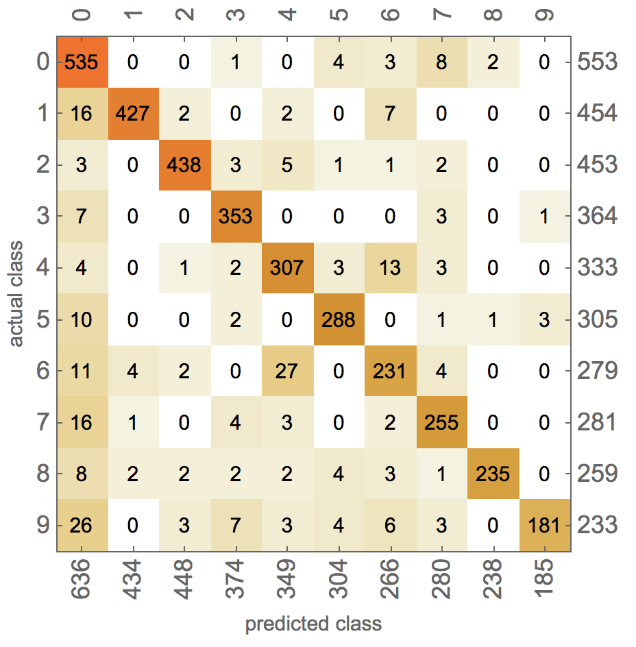
With 92.5% this is quite accurate and also much faster than the competitor product. The confusion plot shows that it is a very reasonable accuracy - in particular when considering that native speakers have problems identifying the glyphs.

cmstandard["ConfusionMatrixPlot"]

Here are some glyphs that the Classifier identified as class "0":

cmstandard["Examples" -> {0, 0}][[1 ;; 20]]

They look quite diverse, but so does the original set:

RandomSample[Select[trainingset, #[[2]] == 0 &], 20]

It is quite impressive that the Classify function manages to achieve this level of accuracy. We can, however, do better!

Machine Learning (NetTrain)

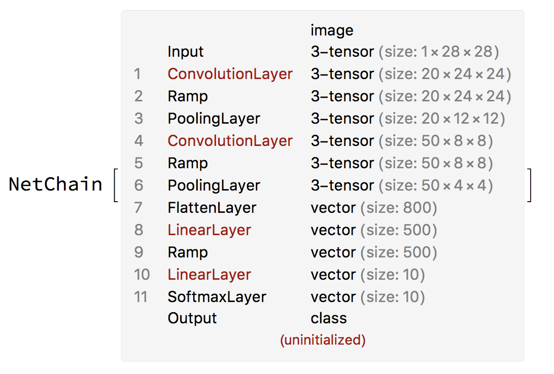
We can improve the accuracy by training our own custom made network, which in this case will be the standard net that is often used for the MNIST dataset in Mathematica. It turns out that we do not even need a GPU for the training.

lenet = NetChain[{ConvolutionLayer[20, 5], Ramp, PoolingLayer[2, 2], 
   ConvolutionLayer[50, 5], Ramp, PoolingLayer[2, 2], FlattenLayer[], 
   500, Ramp, 10, SoftmaxLayer[]}, 
  "Output" -> NetDecoder[{"Class", Range[0, 9]}], 
  "Input" -> NetEncoder[{"Image", {28, 28}, "Grayscale"}]]

This we can then train:

lenet = NetTrain[lenet, trainingset, ValidationSet -> testset, MaxTrainingRounds -> 20];

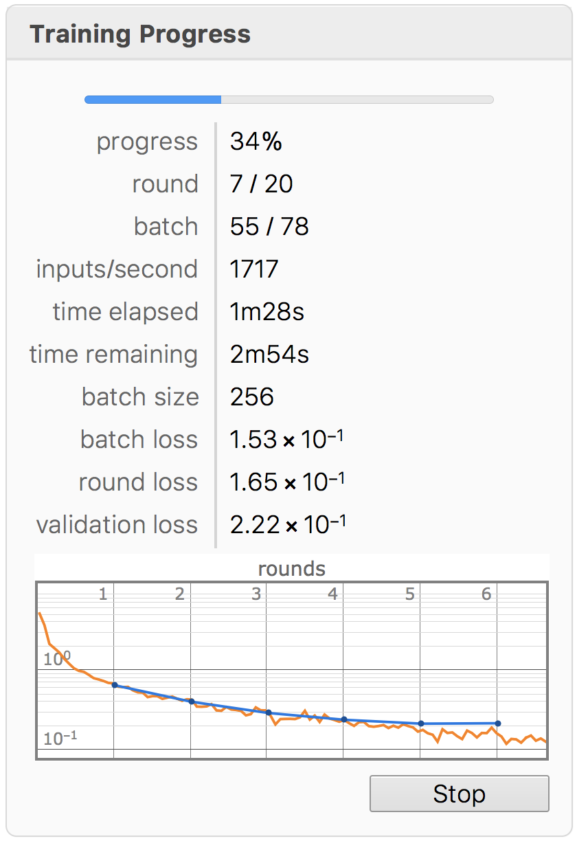
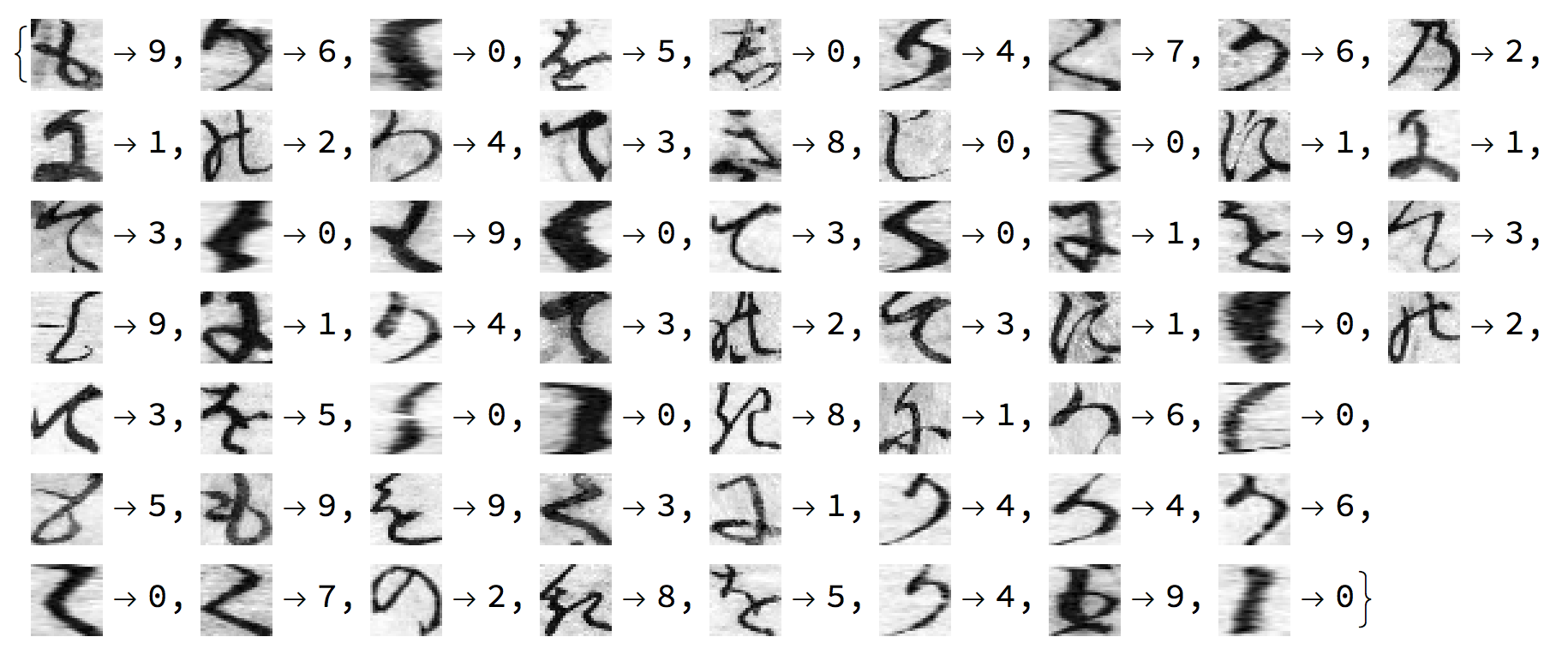
The training is done in about 4:30 minutes, but it appears that 20 training rounds are not necessary. Here are some results when applying the classifier:

imgs = Keys@RandomSample[testset, 60]; Thread[imgs -> lenet[imgs]]

Let's see how well it does:

cm = ClassifierMeasurements[lenet, testset]
cm["ConfusionMatrixPlot"]

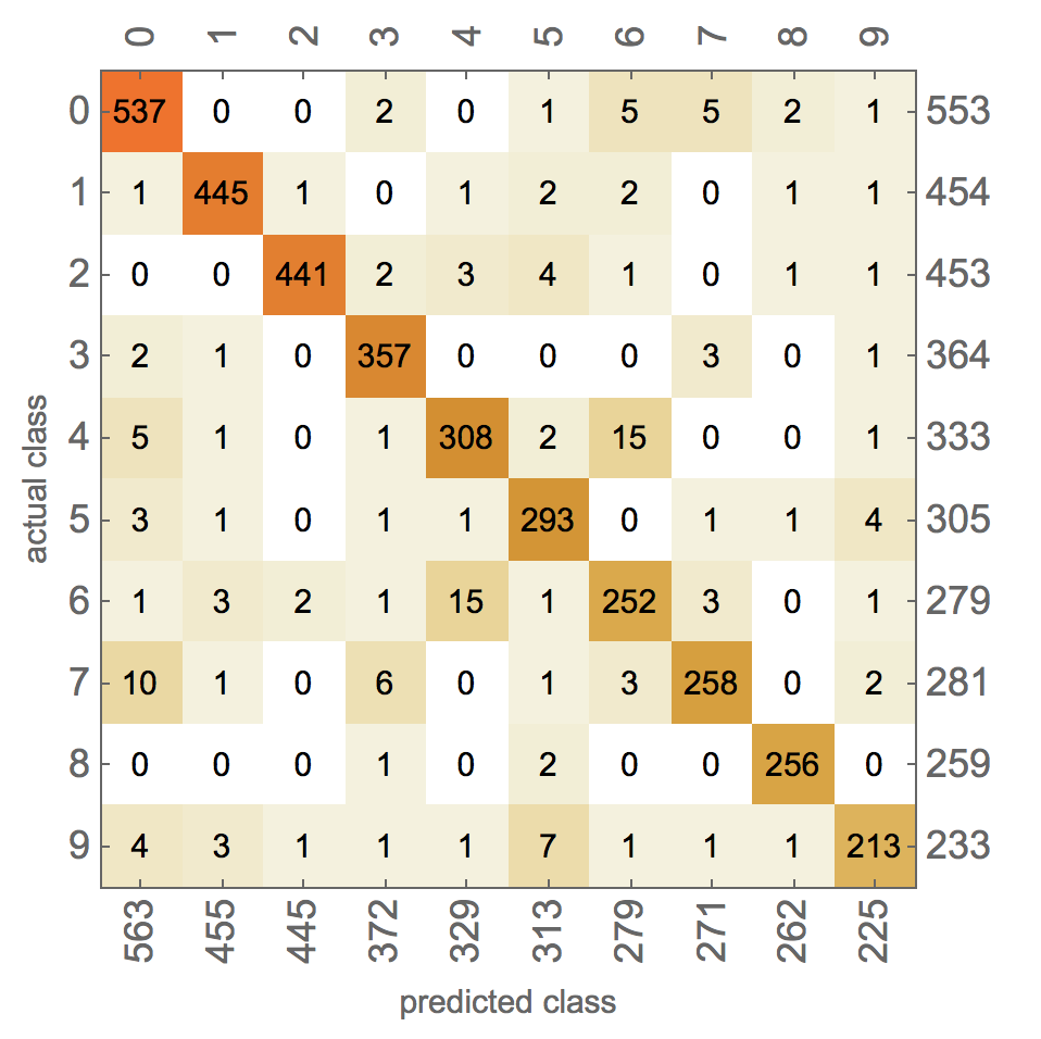
This corresponds to an accuracy of

cm["Accuracy"]

95.6%, which is really impressive given the dataset. The following table illustrates the difficulty:

Grid[Table[
Prepend[Select[trainingset, #[[2]] == k &][[1 ;; 10]][[All, 1]], 
ImageResize[calisymbols[[k + 1]], 28]], {k, 0, 9}], Frame -> All, 
Background -> {{Red}, None}]

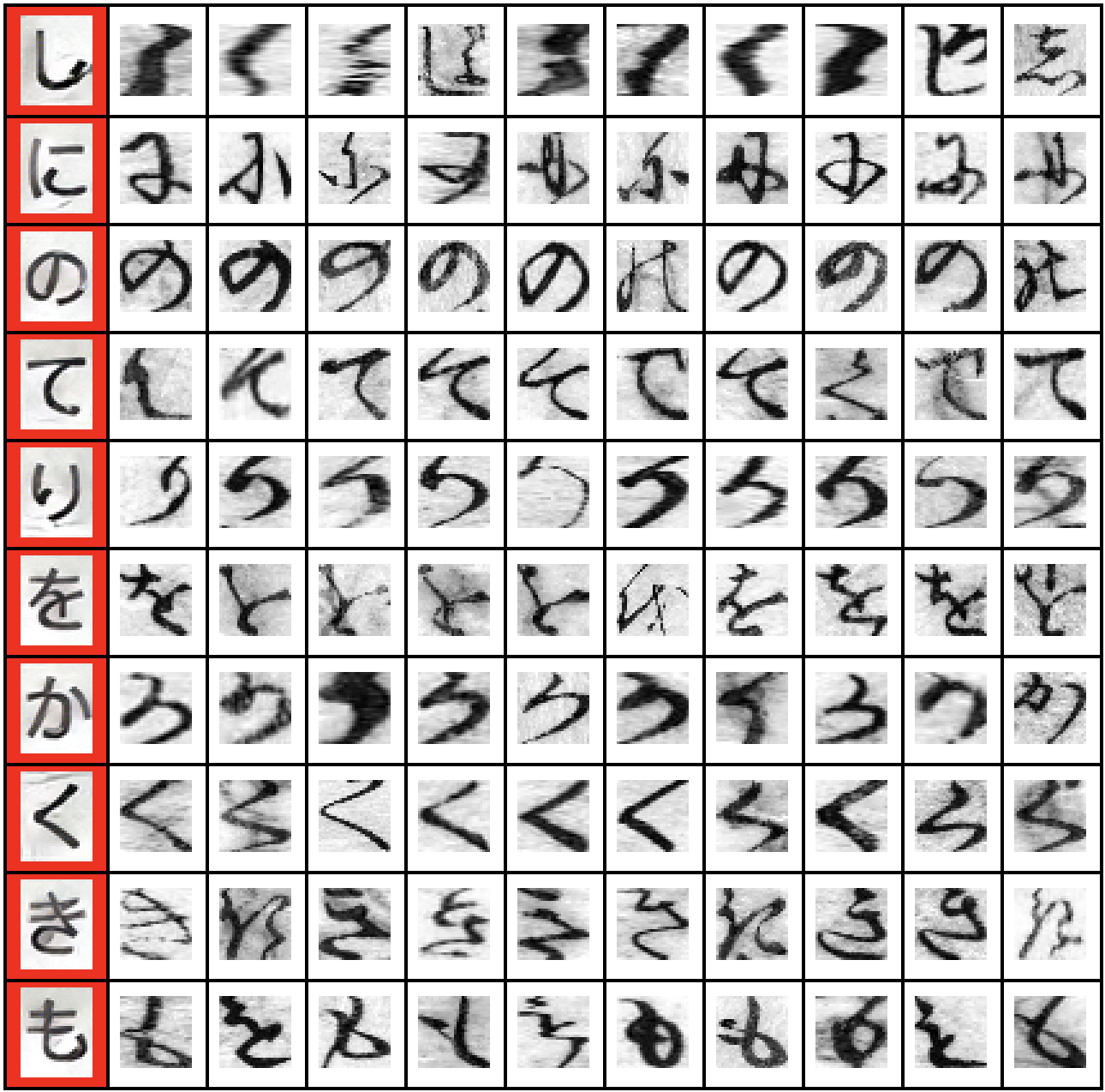
The first (red) column is derived from the glyph based on the character code - using our "calligraphy-style". The remaining columns show items from the training set, i.e. glyphs that were manually classified to belong to the given group.

Conclusion

I do not speak/read Japanese and have no more than Wikipedia knowledge about the Edo period. I still find it quite amazing that using the Wolfram Language's high level Classify function and one of the pre-implemented networks, we can achieve quite a remarkable classification. I am sure that the network can be improved. I would also like to see a more complete dataset with more than 10 different symbols.