Hello everyone, this is my first post in Wolfram community, so I am quite excited about it!
I got interested in the neural network functionalities, after attending a talk, right when version 11.0.0 of Mathematica was about to release (so about one and half years back). Since then, I have just been self-teaching myself about neural networks using various resources available online and Wolfram Language documentation. What really helped me with this current post (project) is the ease with which one can implement a seemingly complicated network in Wolfram Language, the level of automation which NetTrain handles behind the scenes (batch sizes, methods, learning rates, initializations... and the list can go on), and the simplicity with which we can all stitch (chain) it together and run (essentially Shift+Enter) using Wolfram Language.
So in this post, I have tried to implement SegNet ( https://arxiv.org/pdf/1511.00561.pdf ). It is a convolution neural network for a semantic pixel-wise segmentation. The encoder network is identical to the first 13 layers of the VGGNetwork, identical because each convolution layer is followed by a batch-normalization. The decoder upsamples the image obtained from the encoder, using Max pooling. (please note that this encoder, is not the same as NetEncoder and NetDecoder functionality in Wolfram Language). A snippet from the paper cited above shows the layer organization 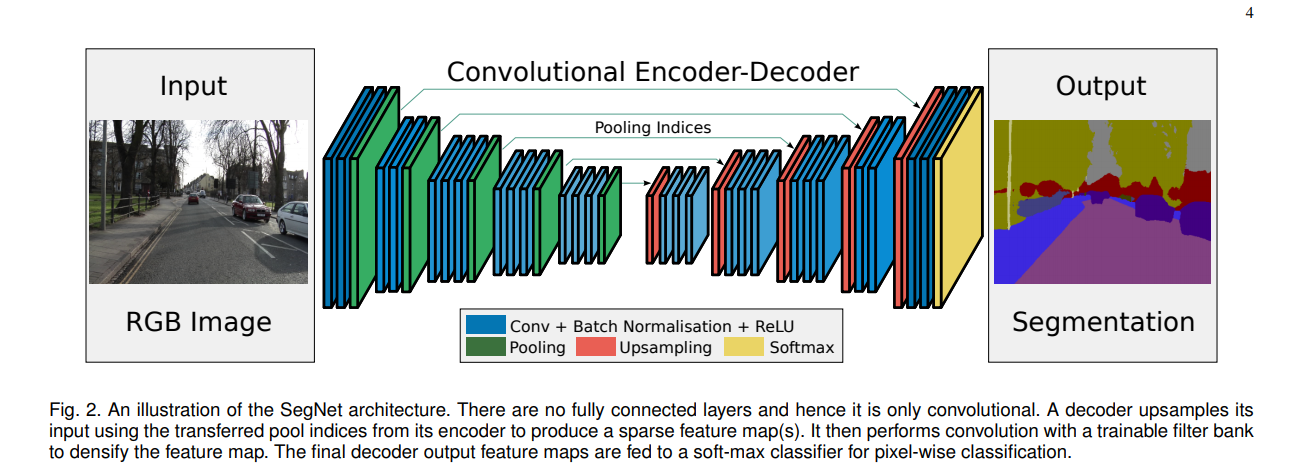
So let's take a step by step approach to build this network: let's start with the encoder network. To build the networks, I directly referred to the Caffe prototxt files and tried to reproduce the same in Wolfram Language. So if we see the prototxt files that it has a structure of the layers, and these structures have a repetitive pattern. Taking use of that, we can build the encoder in a nicer neater way:
encChain[index_, nLayers_, nChannels_] := Module[{tags, names, layers},
  tags = Table[ToString[index] <> "_" <> ToString[j], {j, nLayers}];
  names = Append[
    Flatten[{"conv" <> #, "conv" <> # <> "bn", "relu" <> #} & /@
      tags], "pool" <> ToString[index]];
  layers = Append[
    Flatten@Table[{ConvolutionLayer[nChannels, {3, 3},
        "PaddingSize" -> {1, 1}], BatchNormalizationLayer[],
       ElementwiseLayer[Ramp]}, {nLayers}],
    PoolingLayer[{2, 2}, "Stride" -> {2, 2}]];
  AssociationThread[names -> layers]]

encoder = NetChain[Join[
   encChain[1, 2, 64],
   encChain[2, 2, 128],
   encChain[3, 3, 256],
   encChain[4, 3, 512],
   encChain[5, 3, 512]],
  "Input" ->
   NetEncoder[{"Image", {256, 256}}]]
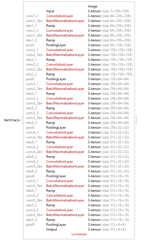
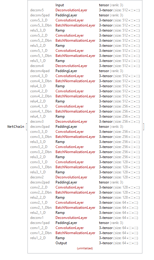
Next we can move to the decoder section of the network. This is similar to the encoder section, and it also contains the patterns which we had seen in the encoder, only now we need to add the appropriate padding, after the upsampling using a DeconvolutionLayer. Here is a decoder which is similar (if not the same) as the prototxt of the Segnet found in literature
decChain[index_, nLayersmax_, nLayersmin_, nChannels_] :=
 Module[{tags, names, layers, nlayers},
  nlayers = nLayersmax - nLayersmin + 1;
  tags = Table[
    ToString[index] <> "_" <> ToString[j] <> "_" <> "D", {j,
     nLayersmax, nLayersmin, -1}];
  names = Flatten@
    Append[{"deconv" <> ToString[index],
      "deconv" <> ToString[index] <> "pad"},
     Flatten[{"conv" <> #, "conv" <> # <> "bn", "relu" <> #} & /@
       tags]]; layers =
   Flatten@Append[{DeconvolutionLayer[nChannels, {3, 3},
       "Stride" -> 2, "PaddingSize" -> 1],
      PaddingLayer[{{0, 0}, {0, 1}, {0, 1}}]},
     Flatten@Table[{ConvolutionLayer[nChannels, {3, 3},
         "PaddingSize" -> {1, 1}], BatchNormalizationLayer[],
        ElementwiseLayer[Ramp]}, {nlayers}]];
  AssociationThread[names -> layers]]

decChain2[index_, nLayersmax_, nLayersmin_, nChannels_] :=
 Module[{tags, names, layers, nlayers},
  nlayers = nLayersmax - nLayersmin + 1;
  tags = Table[
    ToString[index] <> "_" <> ToString[j] <> "_" <> "D", {j,
     nLayersmax, nLayersmin, -1}];
  names = Flatten[{"conv" <> #, "conv" <> # <> "bn", "relu" <> #} & /@
      tags]; layers =
   Flatten@Table[{ConvolutionLayer[nChannels, {3, 3},
       "PaddingSize" -> {1, 1}], BatchNormalizationLayer[],
      ElementwiseLayer[Ramp]}, {nlayers}];
  AssociationThread[names -> layers]]

decoder = NetChain[Join[
   decChain[5, 3, 1, 512],
   decChain[4, 3, 2, 512],
   decChain2[4, 1, 1, 256],
   decChain[3, 3, 2, 256],
   decChain2[3, 1, 1, 128],
   decChain[2, 2, 2, 128],
   decChain2[2, 1, 1, 64],
   decChain[1, 2, 2, 64]]]
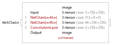
The last step would be to just put it all together, chain them with the final layer depending on the application. Since in this code (project), I just wanted to obtain a final image (pixel classified according to the object class), I kept the Output as an image.
chain = NetChain[{encoder, decoder,
   ConvolutionLayer[3, {3, 3}, "PaddingSize" -> 1,
    "Input" -> {64, 256, 256},
    "Output" ->
     NetDecoder[{"Image"}]]}]
Now, as a proof of concept, the network was trained on images from the EarthObject dataset: http://www2.isprs.org/potsdam-2d-semantic-labeling.html. This dataset was chosen because there was already a similar trained network in Caffe https://github.com/nshaud/DeepNetsForEO, and I just wanted to implement the same in Wolfram Language.
The dataset consists of images of dimensions {6000,6000}. They were appropriately divided into training, validation, and test images. Once done, they were imported, resized to {2048,2048} images, and partitioned into {256,256} sized images so that I could feed it into the modest-sized GPU that I had. So each image created a set of 64 images.
The final last step would be to train it, for training this network, a very modest GPU was used (just a laptop, 4GB graphics card), with Images of dimensions {256,256}, BatchSize 10.
dir = SetDirectory[NotebookDirectory[]];
trained=NetTrain[chain, traindata, ValidationSet -> valdata,
 MaxTrainingRounds -> 1000, TargetDevice -> "GPU",
 BatchSize -> 10,
 TrainingProgressCheckpointing -> {"Directory", dir,
   "Interval" -> Quantity[30, "Minutes"]}]
Once the network was trained to some extent (it was not trained completely, since the Validationloss had not plateaued yet), I was impatient to look at results (this is indeed my first neural net exploratory project).
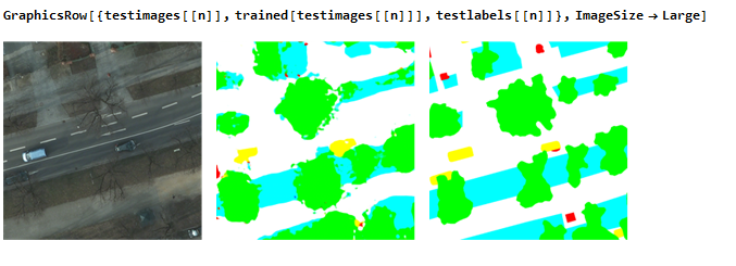
The above shows roads, cars, and trees as trained by the network. The first is the actual image, second image is the trained classes, while the third is the actual label (ground truth)
I am still working on an efficient way to do error analysis. Please feel free to provide me feedback, so that I can improve on this code, do efficient error analysis, or even suggestions for other nets that I can try to code (implement) in the Wolfram Language. I am aware of the CityScapes dataset (https://www.cityscapes-dataset.com/) and Synthia dataset, which might be interesting applications of this net, and they are still work in progress (limited by the GPU availability)
P.S. This was trained for research/leisure purposes only, and cannot be used for commercial use.