Message Boards Message Boards

1
|
6937 Views
|
6 Replies
|
3 Total Likes
View groups...
Share
Share this post:

Place a ContourPlot under a Plot3D?

Posted 6 years ago

I would like to combine a 3-dimensional graph of a function with its 2-dimensional contour-plot underneath it in a professional way. But I have no idea how to start, I try this:

W[s_, b_, q_, 
  p_] := (1/\[Pi]) Exp[-(p^2) + 
    I*Sqrt[2] p (b - Conjugate[s]) - (1/
       2)*((Abs[s])^2 + (Abs[b])^2) - (q^2) + 
    Sqrt[2]*q*(b + Conjugate[s]) - (Conjugate[s]*b)]

Wpsi[\[Alpha]_, q1_, p1_, q2_, p2_] := 
 Np[\[Alpha]]^2 (W[\[Alpha], \[Alpha], q1, p1]*
     W[\[Alpha], \[Alpha], q2, p2] + 
    W[\[Alpha], -\[Alpha], q1, p1]*W[\[Alpha], -\[Alpha], q2, p2] + 
    W[-\[Alpha], \[Alpha], q1, p1]*W[-\[Alpha], \[Alpha], q2, p2] + 
    W[-\[Alpha], -\[Alpha], q1, p1]*W[-\[Alpha], -\[Alpha], q2, p2])

plot3D = Plot3D[Wpsi[1, 0, p1, 0, p2], {p2, -2, 2}, {p1, -2, 2}, 
   PlotTheme -> "Scientific", PlotPoints -> 60, PlotRange -> All, 
   ColorFunction -> Hue, PlotLegends -> Automatic, Mesh -> None];
cntplot = 
  ContourPlot[Wpsi[1, 0, p1, 0, p2], {p2, -2, 2}, {p1, -2, 2}, 
   PlotRange -> All, Contours -> 20, Axes -> False, PlotPoints -> 30, 
   PlotRangePadding -> 0, Frame -> False, ColorFunction -> Hue];
gr = Graphics3D[{Texture[cntplot], EdgeForm[], 
    Polygon[{{-2, -2, -0.4}, {2, -2, -0.4}, {2, 2, -0.4}, {-2, 
       2, -0.4}}, 
     VertexTextureCoordinates -> {{0, 0}, {1, 0}, {1, 1}, {0, 1}}]}, 
   Lighting -> "Naturel"];

Show[plot3D, gr, PlotRange -> All, BoxRatios -> {1, 1, .6}, 
 FaceGrids -> {Back, Left}]

that gives: graph 
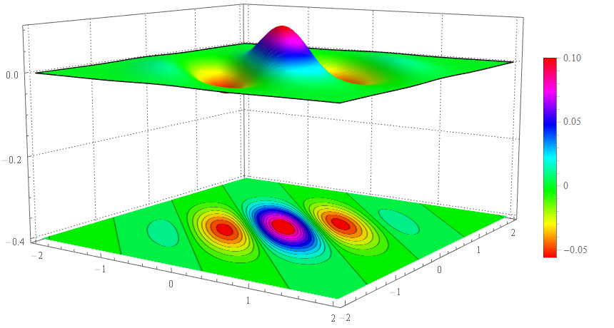
it is not good for me, I want some think like this: needs

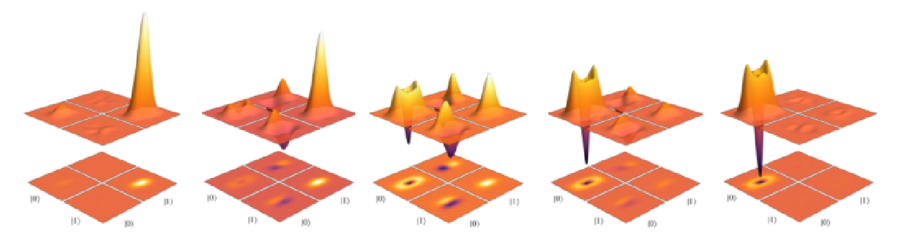
Are i can do it by mathematica ?

POSTED BY: Ziane Mustapha
6 Replies

Function not defined Np[\[Alpha]]^2

The function Np[\[Alpha]]^2 is not defined . I put Np[\[Alpha]]^2=1. We can use this code

W[s_, b_, q_, 
  p_] := (1/\[Pi]) Exp[-(p^2) + 
    I*Sqrt[2] p (b - Conjugate[s]) - (1/
       2)*((Abs[s])^2 + (Abs[b])^2) - (q^2) + 
    Sqrt[2]*q*(b + Conjugate[s]) - (Conjugate[s]*b)]

Wpsi[\[Alpha]_, q1_, p1_, q2_, 
  p2_] := (W[\[Alpha], \[Alpha], q1, p1]*
    W[\[Alpha], \[Alpha], q2, p2] + 
   W[\[Alpha], -\[Alpha], q1, p1]*W[\[Alpha], -\[Alpha], q2, p2] + 
   W[-\[Alpha], \[Alpha], q1, p1]*W[-\[Alpha], \[Alpha], q2, p2] + 
   W[-\[Alpha], -\[Alpha], q1, p1]*W[-\[Alpha], -\[Alpha], q2, p2])

plot3D[x_] := 
  Plot3D[Wpsi[x, 0, p1, 0, p2], {p2, -2, 2}, {p1, -2, 2}, 
   PlotPoints -> 60, PlotRange -> All, ColorFunction -> Automatic, 
   Mesh -> None, Axes -> False, Boxed -> False];
cntplot[x_] := 
  ContourPlot[Wpsi[x, 0, p1, 0, p2], {p2, -2, 2}, {p1, -2, 2}, 
   PlotRange -> All, Contours -> 20, Axes -> False, PlotPoints -> 30, 
   PlotRangePadding -> 0, Frame -> False, ColorFunction -> Automatic];
gr[x_] := 
  Graphics3D[{Texture[cntplot[x]], EdgeForm[], 
    Polygon[{{-2, -2, -1}, {2, -2, -1}, {2, 2, -1}, {-2, 2, -1}}, 
     VertexTextureCoordinates -> {{0, 0}, {1, 0}, {1, 1}, {0, 1}}]}, 
   Lighting -> "Naturel", Boxed -> False];
s[x_] := Show[plot3D[x], gr[x], ViewPoint -> {2, -2, 1}, 
  Boxed -> False, BoxRatios -> {1, 1, 1}]
Table[s[x], {x, .5, 2, .5}]

fig1

A small variation on Alexander's solution:

gr2[x_] := 
 Graphics3D[
  Cases[cntplot[x], 
   GraphicsComplex[pts_, others___] :> 
    GraphicsComplex[Map[Append[-1], pts], others], All]]

This way the contour plot does not get rasterized. You can see the difference by enlarging:

With[{r = .1},
 {Show[gr[1], 
   PlotRange -> {r + r {-1, 1}, r + r {-1, 1}, -1 + r {-1, 1}}],
  Show[gr2[1], 
   PlotRange -> {r + r {-1, 1}, r + r {-1, 1}, -1 + r {-1, 1}}]}]
POSTED BY: Gianluca Gorni

There's SliceContourPlot3D. Just set the slice to be the bottom plane (too bad Bottom does not work automatically since this is a common application!):

ClearAll[myplot];
SetAttributes[myplot, HoldAll];
myplot[f_, x_List, y_List, z : {zsym_, z1_, z2_}, opts___?OptionQ] :=
 Show[
   SliceContourPlot3D[f, zsym == z1, x, y, z, Evaluate@FilterRules[{opts}, Options@SliceContourPlot3D]],
   Plot3D[f, x, y, Evaluate@FilterRules[{opts}, Options@Plot3D], PlotRange -> {z1, z2}]
   ];

myplot[Cos[2 (x + y)]/(2 + x^4 - x y + y^4), {x, -2, 2}, {y, -2, 2}, {z, -2, 1}, ColorFunction -> Hue]

enter image description here

POSTED BY: Michael Rogers

Please see relevant discussion: "Placing a ContourPlot under a Plot3D "

http://community.wolfram.com/groups/-/m/t/1148582

POSTED BY: Moderation Team

Thank you, this very interesting design is being discussed on http://community.wolfram.com/groups/-/m/t/1148582 As I understand it, we are discussing not just "Placing a ContourPlot under a Plot3D ", but a special design that the author of the topic suggested. And then how this design is implemented in Mathematica codes. In the discussion on http://community.wolfram.com/groups/-/m/t/1148582 there is nothing about it.

Reply to this discussion
Community posts can be styled and formatted using the Markdown syntax.
Reply Preview
Attachments
Remove
or Discard

Group Abstract Group Abstract