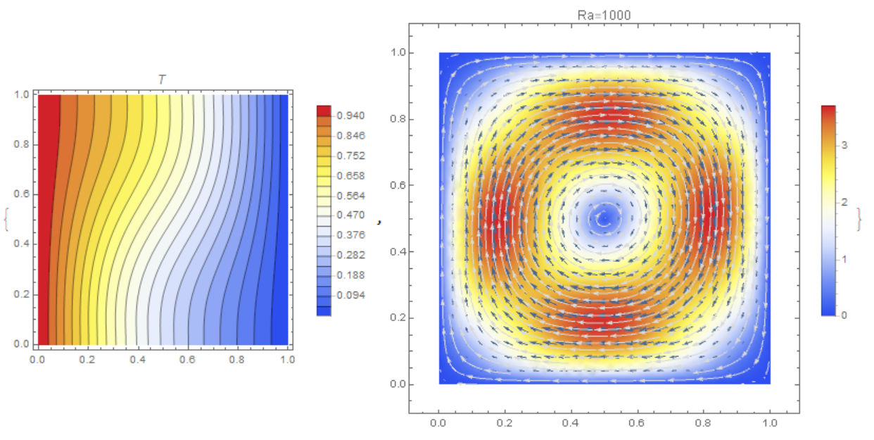
I tested this method of solution on the problems of natural convection. Here we give three tests for the problem of natural convection of air in a rectangular cavity with a Rayleigh number of
$Ra=10^3,10^4, 10^5$. On the side walls of the cavity a constant temperature difference is maintained, the upper and lower walls are thermally insulated. We use the Boussinesq approximation. As a standard, we use the data from the article:
Vahl Davis, G.de (1983) : Natural convection of air in a square cavity : A bench mark numerical solution. Int. J. Numer. Methods Fluids 3, 249-264.
Coincidence in all three tests is generally good. Thus, we showed the application of the method for solving the problems of thermal convection in the case of laminar flows.
A system of equations describing free convection
$\nabla .\vec u=0, \frac{d\vec u}{dt}=Pr\nabla ^2\vec u -RaPrT\frac {\vec g}{g}$
$\frac {dT}{dt}=\nabla^2T$
$ d/dt =\partial/\partial t +(\vec u .\nabla )$
$\vec u$ is velocity field vector,
$T$ - temperature,
$\vec g $ - gravity vector,
$Pr$ - the Prandtl number,
$Ra$ - the Rayleigh number.
Code for the case
$Pr=0.71, Ra=10^3$:
K = 100; Pr0 = .71; Ra = 10^3; R = Ra*Pr0; t0 = 1/100; a = 0;
\[CapitalOmega] = ImplicitRegion[0 <= x <= 1 && 0 <= y <= 1, {x, y}];;
UX[0][x_, y_] := 0;
VY[0][x_, y_] := 0;
\[CapitalRho][0][x_, y_] := 0;
TK[0][x_, y_] := 0; TX[0][x_, y_] := 0;
Do[
  {UX[i], VY[i], \[CapitalRho][i], TK[i], TX[i]} =
   NDSolveValue[{{Inactive[
           Div][({{-\[Mu], 0}, {0, -\[Mu]}}.Inactive[Grad][
             u[x, y], {x, y}]), {x, y}] + D[p[x, y], x] +
         UX[i - 1][x, y]*D[u[x, y], x] +
         VY[i - 1][x, y]*D[u[x, y], y] + (u[x, y] - UX[i - 1][x, y])/
          t0 - R*T[x, y]*Sin[a],
        Inactive[
           Div][({{-\[Mu], 0}, {0, -\[Mu]}}.Inactive[Grad][
             v[x, y], {x, y}]), {x, y}] + D[p[x, y], y] +
         UX[i - 1][x, y]*D[v[x, y], x] +
         VY[i - 1][x, y]*D[v[x, y], y] -
         R*T[x, y]*Cos[a] + (v[x, y] - VY[i - 1][x, y])/t0,
        D[u[x, y], x] + D[v[x, y], y]} == {0, 0, 0} /. \[Mu] -> Pr0, {
      DirichletCondition[{p[x, y] == 0}, y == 1 && x == 1],
      DirichletCondition[{u[x, y] == 0, v[x, y] == 0},
       y == 0 || y == 1]}, {UX[i - 1][x, y]*D[T[x, y], x] +
        VY[i - 1][x, y]*D[T[x, y], y] + (T[x, y] - TK[i - 1][x, y])/
         t0 - (D[T[x, y], x, x] + D[T[x, y], y, y]) ==
       NeumannValue[0, y == 0 || y == 1],
      DirichletCondition[{u[x, y] == 0, v[x, y] == 0, T[x, y] == 1},
       x == 0],
      DirichletCondition[{u[x, y] == 0, v[x, y] == 0, T[x, y] == 0},
       x == 1]}}, {u, v, p, T,
\!\(\*SuperscriptBox[\(T\),
TagBox[
RowBox[{"(",
RowBox[{"1", ",", "0"}], ")"}],
Derivative],
MultilineFunction->None]\)}, {x, y} \[Element] \[CapitalOmega],
    Method -> {"FiniteElement",
      "InterpolationOrder" -> {u -> 2, v -> 2, p -> 1, T -> 2},
      "MeshOptions" -> {"MaxCellMeasure" -> 0.001}}], {i, 1, K}];
{ContourPlot[TK[K][x, y], {x, y} \[Element] \[CapitalOmega],
PlotLegends -> Automatic, Contours -> 20, PlotPoints -> 25,
ColorFunction -> "TemperatureMap", AxesLabel -> {"x", "y"},
PlotLabel -> T],
StreamDensityPlot[{UX[K][x, y],
VY[K][x, y]}, {x, y} \[Element] \[CapitalOmega],
StreamPoints -> Fine, StreamStyle -> LightGray,
PlotLegends -> Automatic, VectorPoints -> Fine,
ColorFunction -> "TemperatureMap", PlotLabel -> Row[{"Ra=", Ra}]]}

MaximalBy[Table[{x, VY[K][x, .5]}, {x, 0, 1, .0001}], Last]

 {{0.1787, 3.69762}}

(*BenchmarkCase={x=0.178,vmax=3.697}*)

 MaximalBy[Table[{y, UX[K][0.5, y]}, {y, 0, 1, .0001}], Last]

 {{0.8132, 3.64937}}

 (*BenchmarkCase={y=0.813,umax=3.649}*)


 MaximalBy[Table[{y, -TX[K][0, y]}, {y, 0, 1, 0.0001}], Last]

 {{0.0909, 1.50724}}

 (*BenchmarkCase={y=0.092,Numax=1.505}*)

 NuAv =
 NIntegrate[
  UX[K][x, y]*TK[K][x, y] - TX[K][x, y], {x, 0, 1}, {y, 0, 1},
  WorkingPrecision -> 5]

 1.1159

 (*BenchmarkCase=1.118*)


 Nu0 =  NIntegrate[-TX[K][0, y], {y, 0, 1}, WorkingPrecision -> 5]

 1.1182

(*BenchmarkCase=1.117*)

 Nu05 =
 NIntegrate[UX[K][.5, y]*TK[K][.5, y] - TX[K][0.5, y], {y, 0, 1},
  WorkingPrecision -> 5]

1.1179

 (*BenchmarkCase=1.118*)

MinimalBy[Table[{y, -TX[K][0, y]}, {y, 0, 1, 0.0001}], Last]

 {{1., 0.691182}}

 (*BenchmarkCase={y=1,Numin=0.692}*)
 Attachments:


