When plotting analytic expressions with such functions like Plot3D, ContourPlot, etc. we most commonly use
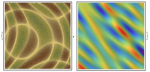
color gradients to beautify the graphs. Here are examples for "SouthwestColors" and "Rainbow" gradient color schemes:
{ReliefPlot[Table[RandomReal[] (Sin[x + y^2] + Sin[x^2 + 3 y]), {x, -3, 3, .01}, {y, -3, 3, .01}],
ColorFunction -> ColorData["SouthwestColors"]],
ReliefPlot[Table[Evaluate[Sum[Sin[RandomReal[4, 2].{x, y}], {5}]], {x, 0, 10, .05}, {y, 0, 10, .05}],
ColorFunction -> ColorData["Rainbow"]]}
There are 51 built in gradients in Mathemtica.
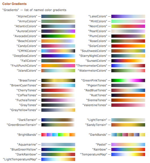
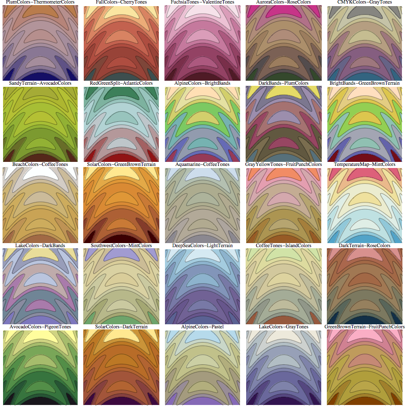
We could have at least 51^2 if we would learn how to blend them. Define a blending function
mixer[grad1_, grad2_][m_, x_] := Blend[{ColorData[grad1][x], ColorData[grad2][x]}, m]
where m is the blending ratio. Now we can mix randomly color gradients at 0.5 even blending ratio to see what kind of colors palettes we get:
g[grad1_, grad2_] := ContourPlot[y + Sin[x^2 + 3 y], {x, -3, 3}, {y, -3, 3},
ColorFunction -> (mixer[grad1, grad2][.5, #] &), Frame -> False,
PlotRangePadding -> 0, PlotLabel -> Style[grad1 <> "-" <> grad2, 10]]
GraphicsGrid[Partition[ParallelTable[g[RandomChoice[ColorData["Gradients"]],
RandomChoice[ColorData["Gradients"]]], {25}], 5], Spacings -> 0, ImageSize -> 800]
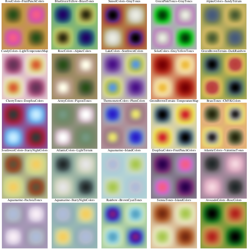
We could also blend at a changing ration, so that at min we have one color gradient and at max the other one, with smooth change in between.
f[grad1_, grad2_] := DensityPlot[Sin[x] Sin[y], {x, -Pi, Pi}, {y, -Pi, Pi},
ColorFunction -> (mixer[grad1, grad2][#, #] &), Frame -> False,
PlotRangePadding -> 0, PlotLabel -> Style[grad1 <> "-" <> grad2, 10], PlotPoints -> 40]
GraphicsGrid[Partition[ParallelTable[f[RandomChoice[Complement[ColorData["Gradients"], {"BrightBands", "DarkBands"}]],
RandomChoice[Complement[ColorData["Gradients"], {"BrightBands", "DarkBands"}]]], {25}], 5], Spacings -> 0, ImageSize -> 800]
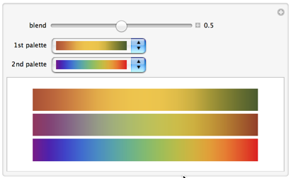
A Manipulate to play with blending:
Manipulate[
GraphicsGrid[{
{DensityPlot[x, {x, 0, 1}, {y, 0, .1}, ColorFunction -> gradients1, AspectRatio -> Automatic, Frame -> False]},
{DensityPlot[x, {x, 0, 1}, {y, 0, .1}, ColorFunction -> (mixer[gradients1, gradients2][m, #] &),
AspectRatio -> Automatic, Frame -> False]},
{DensityPlot[x, {x, 0, 1}, {y, 0, .1}, ColorFunction -> gradients2, AspectRatio -> Automatic, Frame -> False]}
}]
, {{m, .5, "blend"}, 0, 1, Appearance -> "Labeled"}
, {{gradients1, "SandyTerrain", "1st palette"}, (# -> Show[ColorData[#, "Image"], ImageSize -> 100]) & /@ ColorData["Gradients"]}
, {{gradients2, "Rainbow", "2nd palette"}, (# -> Show[ColorData[#, "Image"], ImageSize -> 100]) & /@ ColorData["Gradients"]}]
I think these are pretty nice subtle color palettes. Now I have two questions.
- How do we make the mixer function faster, efficient?
- How do we do the same for "Indexed" discrete color data ColorData["Indexed"] ?


