Message Boards Message Boards

8
|
22038 Views
|
8 Replies
|
13 Total Likes
View groups...
Share
Share this post:

Cobweb plot in Mathematica

Because Mathematica does not have this function (yet) I give here a simple way to produce a cobweb plot: http://en.wikipedia.org/wiki/Cobweb_plot
The code is quite short and does the basics:
 ClearAll[CobwebPlot]
 Options[CobwebPlot]=Join[{CobStyle->Automatic},Options[Graphics]];
 CobwebPlot[f_,start_?NumericQ,n_,xrange:{xmin_,xmax_},opts:OptionsPattern[]]:=Module[{cob,x,g1,coor},
  cob=NestList[f,N[start],n];
  coor = Partition[Riffle[cob,cob],2,1];
  coor[[1,2]]=0;
  cobstyle=OptionValue[CobwebPlot,CobStyle];
  cobstyle=If[cobstyle===Automatic,Red,cobstyle];
  g1=Graphics[{cobstyle,Line[coor]}];
Show[{Plot[{x,f[x]},{x,xmin,xmax},PlotStyle->{{Thick,Black},Black}],g1},FilterRules[{opts},Options[Graphics]]]
]
The function works as follows:
CobwebPlot[f,start,n,xrange,...]
Where 
f is a pure function
start is the starting value
n is number of iterations
xrange is a the range of the plot and should have the form: {xminimum,xmaximum}.

The color of the cobweb can be given by a CobStyle option, additionally one can add other options as well (those of Graphics).

Examples:
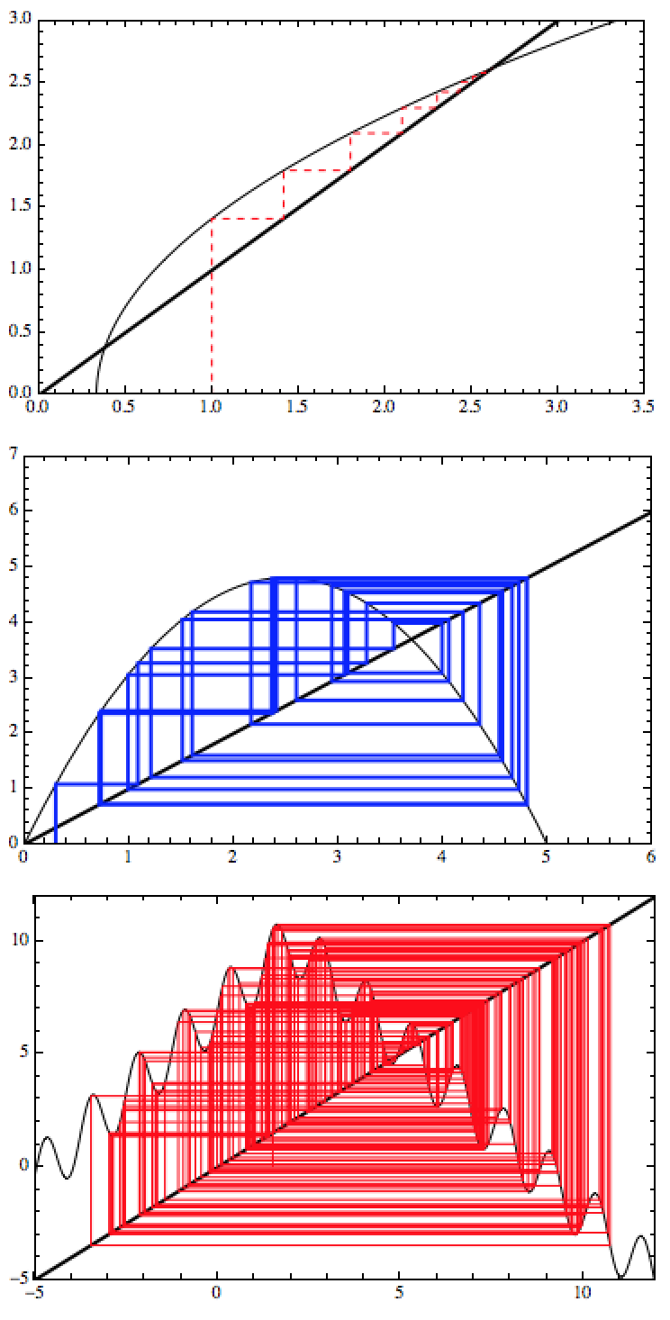
CobwebPlot[Sqrt[3#-1]&,1,40,{0,4},PlotRange->{{0,3.5},{0,3}},Frame->True,Axes->False,CobStyle->Directive[Dashed,Red],PlotRangePadding->None]
CobwebPlot[0.77#(5-#)&,0.3,30,{0,10},PlotRange->{{0,6},{0,7}},Frame->True,Axes->False,CobStyle->Directive[Blue,Thick],PlotRangePadding->None]
CobwebPlot[10-1.5Abs[#-2]+1.35Sin[5#]&,1.5,230,{-5,12},PlotRange->{Automatic,{-5,12}},Frame->True,Axes->False,CobStyle->Red,PlotRangePadding->None]
giving:
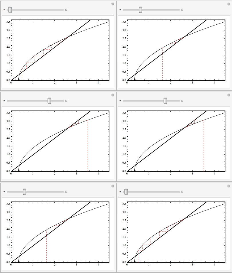
Of course this can be used together with Manipulate like so:
Manipulate[CobwebPlot[Sqrt[3#-1]&,\[Alpha],40,{0,5},PlotRange->{{0,4.5},{0,3.65}},Frame->True,Axes->False,CobStyle->Directive[Dashed,Red],PlotRangePadding->None],{\[Alpha],0.5,4.375}]
giving:

I hope this will be useful. Let me know if you can't get it to work.
POSTED BY: Sander Huisman
8 Replies

Thank you sir.

In the above Code, if I want to Take two initial conditions - one at -1.23 and say other at 2.5, so in Cobweb plots can we show two orbits? I tried following code:

CobwebPlot[
 Piecewise[{{2 # + 3, # <= 0}, {0.7 # + 4, # > 0}}] &, {{-1.23, 40}, {2.5, 40}}, {-15, 15}]

But it didn't work.

Also I want to plot Basin of Attraction plot for the same basic piecewise system.

POSTED BY: Rajanikant Metri

Change the

PlotStyle->{{Thick,Black},Black}]

part to some different colors/style…

POSTED BY: Sander Huisman

Thank You Sir. Can we change the colour of 2x+3 line and 0.7x+4 line? By default it is Black, how to modify the colour of these lines?

POSTED BY: Rajanikant Metri
Show[{CobwebPlot[2 # &, 2, 40, {-15, 15}],
  CobwebPlot[3 # &, 2, 40, {-15, 15}, CobStyle -> Blue]
  }]
POSTED BY: Sander Huisman

Something like:

CobwebPlot[
 Piecewise[{{2 # + 3, # <= 0}, {0.7 # + 4, # > 0}}] &,
 -1.23, 40, {-15, 15}]
POSTED BY: Sander Huisman

Sir, I have piecewise equation

 f = Piecewise[{{a x + m, x <= 0}, {b x + n, x > 0}}]

For this "f" how to plot Cobweb plot? Thank You.

POSTED BY: Rajanikant Metri

Can we use a single plot to represent a cobweb of 1/2 under functions f(x) = 2x and g(x) =3x. So that we can compare their orbit under two distinct functions using one plot.

Great, Sander, I love those! Nice animated GIF too. I wrote a few cobweb Demonstrations myself - see for example the image below. Demonstrations Project have several cobwebs:

POSTED BY: Vitaliy Kaurov
Reply to this discussion
Community posts can be styled and formatted using the Markdown syntax.
Reply Preview
Attachments
Remove
or Discard

Group Abstract Group Abstract