Open in Cloud | Download to Desktop via Attachments Below

The Traditional Ulam Spiral
Although there are some very elegant methods of displaying the Ulam spiral in Mathematica, I wanted one that was slightly more general, with the specific goal of making the Ulam spiral for a hexagonal tiling of the plane.
With that in mind, I adopted the following approach: for the standard rectangular tiling of the plane, the spiral consists of concentric 'shells' of points, each shell containing (2n+1)^2 numbers. Consequently finding which shell a given number is in reduces to taking a square root.
quadlayer[q_] := Ceiling[(Sqrt[q] - 1)/2]
The convention being that the origin is the 'zeroth' shell. Next, we count how many squares 'around' the given shell a number is, just given by taking the difference from the shell underneath it.
quadaround[q_] := q - (2 quadlayer[q] - 1)^2
The method for actually generating the appropriate point comes down to specifying the 'corner' of the shell to start from, and how far along the 'edge' to travel. This is easily determined from the previously determined shell number and 'around' number.
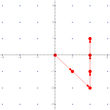
For example, to get the position of 12 in the spiral, we compute that it's in shell 2, so we start at a corner two steps away from the origin. We then compute that it is three steps around this shell, so we travel three steps around the outside.
Use of QuotientRemainder tells us which corner to start at, and how many steps to go
quadpoint[q_] := (quadlayer[q] (Sqrt[2] AngleVector[\[Pi]/2 (#1 - 1/2)])
                                 + (#2) AngleVector[\[Pi]/2 (#1 + 1)]  ) & @@
                  Quiet[QuotientRemainder[quadaround[q], 2 quadlayer[q]]]
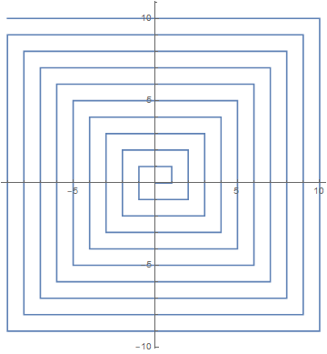
The first part of the vector specifies the corner to start at, and the second specifies how many steps along the edge to take.
ListPlot[quadpoint[#] & /@ Range[400], Joined -> True, AspectRatio -> Automatic]
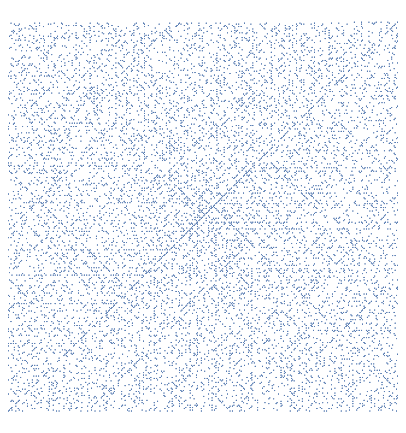
And from there we can generate the ordinary Ulam spiral, or select a starting point, such as p_13=41, which reproduces the rather striking spiral from the wikipedia page on the subject.
ListPlot[quadpoint[# - 40] & /@ (Prime[#] & /@ Range[13, 10000]),
 AspectRatio -> Automatic, Axes -> False]
Generalization
This method of computing where a given integer should end up in the spiral naturally generalizes to m-gons. The first shell will have m points in it, the second will have 2m, etc, so the number of points going up to the n'th layer is just
1+ m n(n-1)/2
And so given an integer, we can again compute which layer it is in, and how many 'around' the layer it goes.
mgonLayer[q_, m_] := Ceiling[1/2 (1 + Sqrt[-8 + m + 8 q]/Sqrt[m])] - 1

maround[q_, m_] := q - (1 + m/2 ((mgonLayer[q, m] - 1) (mgonLayer[q, m])))
And in an exactly analogous way, we can use these to specify where in a shell a given integer should go. A little more geometry is required to figure out where the 'corners' of each layer are, and how long the sides are, but the situation is essentially the same.
mpoint[q_, m_] := (mgonLayer[q, m] AngleVector[(2 \[Pi])/m (#1 - 1)] +
                 #2 2 Sin[\[Pi]/m] AngleVector[2 \[Pi]/m (#1 - 1) + \[Pi]/2 + \[Pi]/m]) & @@
                  Quiet[QuotientRemainder[maround[q, m], mgonLayer[q, m]]]
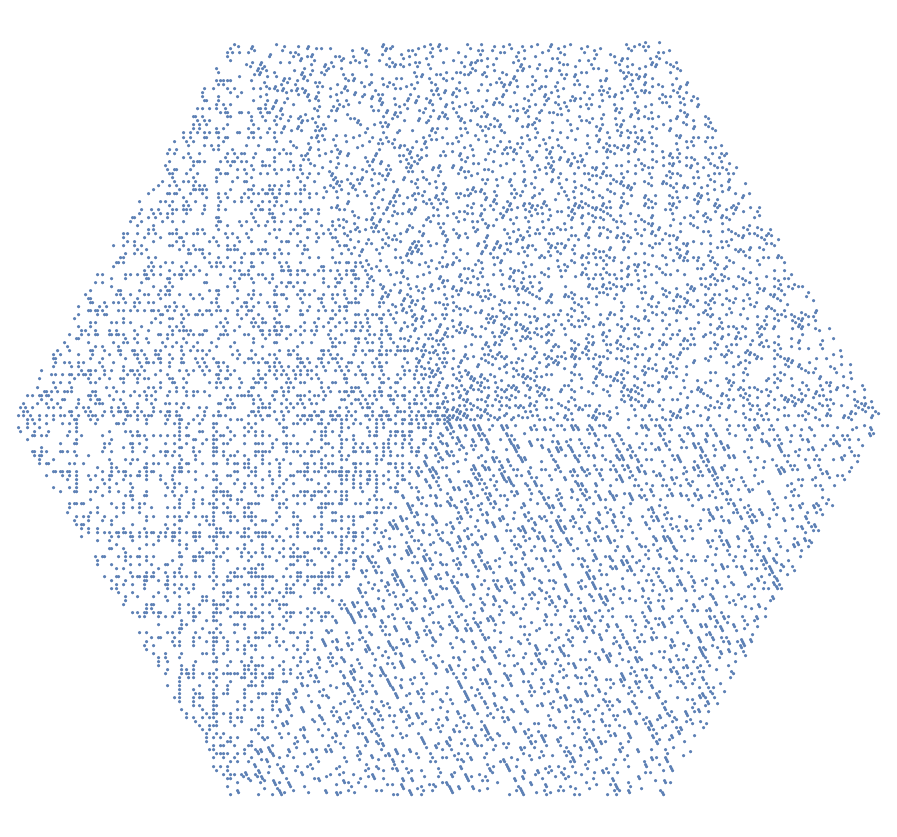
And now we can make Ulam Spirals for any regular polygon we might like
ListPlot[mpoint[#, 6] & /@ (Prime[#] & /@ Range[10000]),
 Axes -> False, AspectRatio -> Automatic]
Another Example: Circular 'tilings'
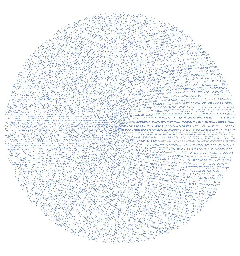
We may also define alternative functions for placing the points. As an example, we may instead have concentric circles of 2m equally spaced points.
mpoint2[q_, m_] := (mgonLayer[q,  m] AngleVector[(2 \[Pi])/(m*mgonLayer[q, m]) (maround[q, m]-1)])

ListPlot[mpoint2[#, 6] & /@ (Prime[#] & /@ Range[10000]), Axes -> False, AspectRatio -> Automatic]
 Some other elegant examples that are possible include displaying ListPlots with pointsize given by number of factors, spirals of prime squares, cubes, etc.
Hopefully this will enable some people to make elegant and visually pleasing Ulam spirals, and related objects.
 Attachments: