Open code in Cloud | Download code to Desktop via Attachments Below
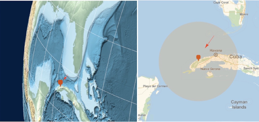
On Feb 1, 2019, a meteor exploded over western Cuba in the area of Viñales where meteorites were found.
In[1]:= meteoritesite =
 Entity["AdministrativeDivision", {"Vinales", "PinarDelRio", "Cuba"}][
  "Position"]

Out[1]= GeoPosition[{22.624, -83.7132}]
At 18:21 UTC, The National Weather Service picked up a radar signature at over 26,000 feet. We can encode this information in a GeoPosition.
In[2]:= finalposition =
 GeoPosition[
  Join[meteoritesite[[1]], {Quantity[26000., "Feet"],
    DateObject[{2019, 2, 1, 18, 21}, TimeZone -> "UTC"]}]]

Out[2]= GeoPosition[{22.624, -83.7132, 7924.8, 3.75803*10^9}]
The American Meteor Society maintains data on recorded observations and stores these in KML format. The results are returned as GeoGraphics.
url = "https://www.amsmeteors.org/members/imo_kml/view_trajectory_kml?\
event_id=513&event_year=2019&avg_start_height=80000&avg_end_height=\
41274.569406897&impact_location_lon=-83.947826518033&impact_location_\
lat=22.6421042042&end_visible_location_lon=-83.216019070606&end_\
visible_location_lat=23.60842985294&start_visible_location_lon=-82.\
505386608356&start_visible_location_lat=24.502650658255";

alldata = Quiet[Import[url, "KML"]]
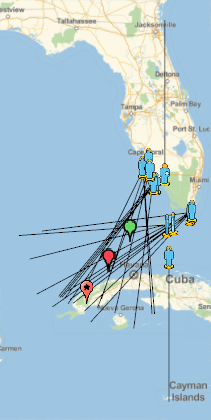
The above diagram shows a fair amount of information, but we will only use a subset of the information. In the above diagram, the lines represent the observed vectors from each observer (13 total). For each observer, a line is drawn from the approximate initial observation direction and another is drawn to the final observation direction for the meteor. From these, an estimated trajectory of the meteor is obtained. The colored disks under each observer position represent the direction of motion of the observed meteor with green traveling from right to left, red indicating left to right, and yellow indicating not enough information to determine direction. The green and red pins mark the start and end of the estimated trajectory, respectively. The orange pin shows the geometric impact point based on the trajectory.
We can also look at the raw data and extract out the more important parts.
In[5]:= kmldata = Quiet[Import[url, {"KML", "Data"}]];
The various layers of the data are mainly individual observations.
In[6]:= "LayerName" /. kmldata

Out[6]= {"Witnesses\\Experience Level 1", "Witnesses\\Experience Level 2", "Witnesses\
\\Experience Level 3", "Lines\\Experience Level 1\\marcia m", \
"Lines\\Experience Level 1\\Tom B", "Lines\\Experience Level 1\\Mary-Sue T", \
"Lines\\Experience Level 1\\Bryce L", "Lines\\Experience Level 1\\Olivia B", \
"Lines\\Experience Level 1\\Susan W", "Lines\\Experience Level 1\\Annette B", \
"Lines\\Experience Level 1\\Renee R", "Lines\\Experience Level 2\\Ashley M", \
"Lines\\Experience Level 2\\David S", "Lines\\Experience Level 3\\Paul B", \
"Lines\\Experience Level 3\\Janie C", "Lines\\Experience Level 3\\Stuart M", \
"Trajectory"}
But, the trajectory can be extracted for a more clear view.
In[7]:= trajectorydata = Select[kmldata, ! FreeQ[#, "Trajectory"] &]

Out[7]= {{"LayerName" -> "Trajectory", "Geometry" -> {Polygon[
GeoPosition[{{23.60842985294, -83.216019070606, 41274.569406897}, {
       24.502650658255, -82.505386608356, 80000}, {
       24.502650658255, -82.505386608356, 0}, {
       23.60842985294, -83.216019070606, 0}, {
       23.60842985294, -83.216019070606, 41274.569406897}}]],
    Point[GeoPosition[{22.6421, -83.9478, 0}]],
    Point[GeoPosition[{24.5027, -82.5054, 0}]],
    Point[GeoPosition[{23.6084, -83.216, 0}]]}, "Labels" -> {},
  "LabeledData" -> {}, "ExtendedData" -> {},
  "PlacemarkNames" -> {"Estimated Trajectory", "Geometric Impact Point",
    "Visible From", "Visible to"}, "Overlays" -> {}, "NetworkLinks" -> {}}}

In[8]:= pointsofinterest =
 Rule @@@ Transpose[({"PlacemarkNames", "Geometry"} /. trajectorydata)[[1]]]

Out[8]= {"Estimated Trajectory" -> Polygon[
GeoPosition[{{23.60842985294, -83.216019070606, 41274.569406897}, {
     24.502650658255, -82.505386608356, 80000}, {
     24.502650658255, -82.505386608356, 0}, {
     23.60842985294, -83.216019070606, 0}, {23.60842985294, -83.216019070606,
     41274.569406897}}]],
 "Geometric Impact Point" -> Point[GeoPosition[{22.6421, -83.9478, 0}]],
 "Visible From" -> Point[GeoPosition[{24.5027, -82.5054, 0}]],
 "Visible to" -> Point[GeoPosition[{23.6084, -83.216, 0}]]}

In[9]:= geometricimpactpoint = ("Geometric Impact Point" /. pointsofinterest)[[1]];

In[10]:= path = SortBy[
   Append[Cases[pointsofinterest, _Point, Infinity][[All, 1]],
    geometricimpactpoint], -#[[1, 2]] &];

In[11]:= estimatedtrajectory =
  GeoPosition[
   DeleteDuplicates[
    SortBy[("Estimated Trajectory" /. pointsofinterest)[[1, 1]], -#[[2]] &]]];
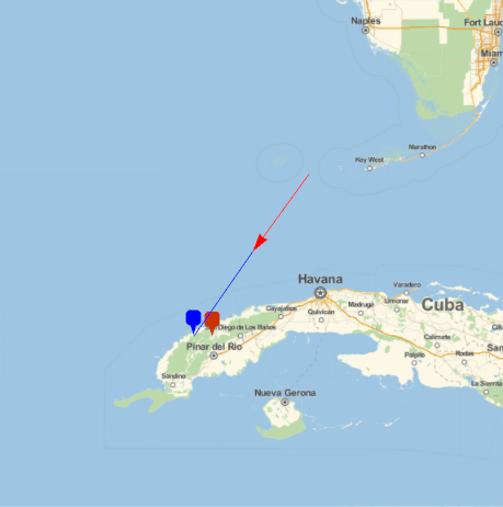
The estimated trajectory can be viewed as a red arrow and is extended toward the geometric impact point as a blue line. The geometric impact point is shown with a blue pin. The site of Viñales meteorites is marked with a red pin.
In[12]:= GeoGraphics[{GeoMarker[finalposition], Blue, Line[path],
  GeoMarker[GeoPosition[geometricimpactpoint], "Color" -> Blue], Red,
  Arrow[estimatedtrajectory]}, GeoRange -> Quantity[200, "Miles"]]
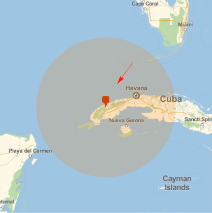
At 26,000 feet elevation, the altitude that the meteor was estimated to have exploded, the only people that could have observed the explosion directly would be within the highlighted area.
GeoGraphics[{Red, Arrow[estimatedtrajectory], GeoMarker[finalposition],
  Orange, GeoVisibleRegion[finalposition]},
 GeoRange -> Quantity[300, "Miles"]]
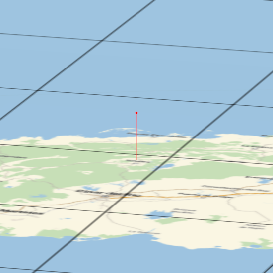
For scale, here is a nearly side view of the affected area. The red dot indicates 26,000 ft elevation, where weather satellites detected an explosion, and a red line is drawn to the ground beneath that point. Grid lines are shown at 20 arc minute intervals.
texture = GeoGraphics[{meteoritesite},
   GeoRange -> Quantity[200, "Kilometers"],
   GeoGridLines -> Quantity[20, "ArcMinutes"], ImageSize -> 1920];

Graphics3D[{ParametricPlot3D[{x, y, 0}, {x, -200, 200}, {y, -200, 200},
    Mesh -> None, PlotStyle -> Texture[texture]][[1]], Red, PointSize[.01],
  Point[{0, 0, QuantityMagnitude[Quantity[26000., "Feet"], "Kilometers"]}],
  Line[{{0, 0, QuantityMagnitude[Quantity[26000., "Feet"], "Kilometers"]}, {0,
      0, 0}}]}, Lighting -> "Neutral", Boxed -> False, Axes -> False,
 SphericalRegion -> True, ViewAngle -> Pi/100, ImageSize -> 550,
 ViewPoint -> {0.94, -3.14, 0.83}, ViewVertical -> {0, 0, 1}]
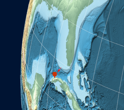
A more 3D looking perspective is available using the forthcoming version 12 of the Wolfram Language and can be simulated as follows. The red arrow indicates the trajectory and the marker pin indicates the location where meteorites were found.
GeoGraphics[{RGBColor[1, 0, 0], GeoMarker[finalposition], Arrowheads[Medium],
  Arrow[estimatedtrajectory]}, GeoRange -> {{25, 28}, {-100, -70}},
 GeoProjection -> {"VerticalPerspective", "Centering" -> {30, -40}},
 GeoGridLines -> Quantity[5, "AngularDegrees"],
 GeoGridLinesStyle -> Directive[Opacity[0.5`], GrayLevel[1]],
 GeoRangePadding -> Full, GeoBackground -> GeoStyling["ReliefMap"],
 Background -> Hue[0.6`, 1, 0.2`],
 PlotRangePadding -> {{0.05`, 0}, {0.03`, 0}}]
 Attachments: