Abstract
In this project, I analyze n-body simulations outputs and their patterns by utilizing different statistical methods, visualization algorithms, and feature extraction techniques. Using an n-body simulation random generation technique, a sample of 5000 different outputs could be generated. By performing feature extraction processes, some interesting visualizations about the different outcomes from the simulations were plotted on a two-dimensional feature space plot. Additional conclusions were made using the distribution of the center-of-mass, and a two-body mass visualization.
Introduction
In physics and astronomy, an N-body simulation is a simulation of a dynamical system of particles, usually under the influence of physical forces, such as gravity. Currently, computing power is sufficient for processing some classes of N-Body simulations, with a small number of bodies, and with a short lapse time. For cases of realistic units such as astronomical units and gigayears, computers can't handle their complexity. A way to prevent this computational complexity difficulty, systems such as "InverseSquare" relativistically treat metric units and unitless quantities mathematically equivalent.
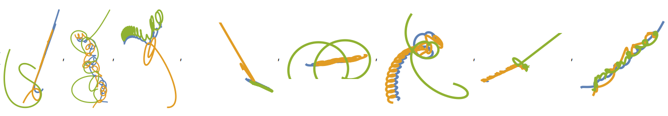
Here are some cases of random n-body simulations, they have an extraordinarily chaotic behavior, and are vulnerable to having their outputs changed with just a few tweaks on their initial states.
CreateRandomBody[] := Block[{},
    <|"Mass" -> RandomReal[{0.01, 0.99}], "Position" -> RandomReal[{-1, 1}, 2], "Velocity" -> RandomReal[{-1, 1}, 2]|>
]

CreateRandomPivot[] := Block[{},
    <|"Mass" -> 1, "Position" -> {0, 0}, "Velocity" -> RandomReal[{-0.25, 0.25}, 2]|>
]

NBodyPlot[data_] := ParametricPlot[Evaluate[data[All, "Position", t]],{t, 0, data["SimulationTime"]}, AspectRatio -> Automatic, Axes -> False, PlotStyle -> {Thickness[0.025], Thickness[0.025], Thickness[0.025]}]

Table[Rasterize[
   NBodyPlot[
    NBodySimulation[
     "InverseSquare", {CreateRandomPivot[], CreateRandomBody[],
      CreateRandomBody[]}, 10]], ImageSize -> Small], 8] // Quiet
For performing the same visualizations and procedures, download the notebook available on this post. The notebook contains all the datasets and files you will need.
HeuristicData = "...";
NBParameters = "...";
NBDPaths = "...";
The "HeuristicData" list contains lists of the heuristic results generated by the "NBodyHeuristics" function (see "Data Generation Procedure"), the "NBParameters" list contains lists of initial parameters, and the "NBDPaths" list contains lists of the final paths of the bodies. Every list is uniform and contains 5000 elements each.
NBParametersDataset = Dataset@NBParameters;

{NBPBodyA, NBPBodyB, NBPBodyC} = Table[NBParametersDataset[[All, t]], {t, 1, 3}];

{allDoubleFalse, allSingleFalse, pivotDiverged, allContained, allDivergent} =
    Table[Join@@Position[HeuristicData, t], {t, {
       {False, True, False} | {False, False, True} | {True, False, False}, {False, True, True} | {True, False, True} | {True, True, False}, {False, True, True}, {True, True, True}, {False, False, False}
       }}];

{allDoubleFalsePoints, allSingleFalsePoints, allContainedPoints, allDivergentPoints, pivotDivergedPoints} =
    Table[Thread[{Normal[NBPBodyB[x, "Mass"]], Normal[NBPBodyC[x, "Mass"]]}], {x, {allDoubleFalse, allSingleFalse, allContained, allDivergent, pivotDiverged}}];

ListPlot[{allContainedPoints, allDivergentPoints, pivotDivergedPoints, allDoubleFalsePoints},PlotStyle -> {RGBColor[0.9, 0.9, 0.9], {PointSize[0.01], Blue}, {PointSize[0.01], Red}, {PointSize[0.01], Orange}}, AspectRatio -> Automatic, PlotTheme -> "Detailed", PlotLegends -> {"All Bodies Contained", "All Bodies Diverged", "Pivot Diverged", "Two Bodies Diverged"}, PlotLabel -> "Masses of the Lightest Objects and Stability", LabelStyle -> {16, GrayLevel[0]}, ImageSize -> {500, 500}]
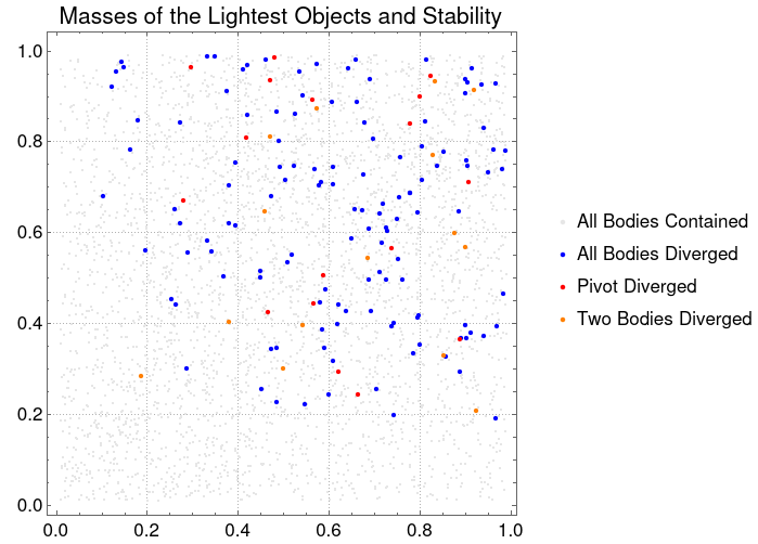
With this plot, we can visualize that there's is a correlation between the lighter bodies masses and the stability of the systems. The lightest bodies have the most stability in their simulations, which means that they are not "catapulted" from the system.
Now, let's calculate the distances between the center of masses using $\frac{\sum _{i=j}^n m_i x_i}{\sum _{i=j}^n m_i}$ as $m_i$ being the mass of the individual bodies and $x_i$ as the positions in space.
centerOfMass = Thread[{Normal@NBParametersDataset[[All, All, "Mass"]], NBDPaths}];

centerOfMasses = Table[(centerOfMass[[n]][[1]]*centerOfMass[[n]][[2]] // Total)/Total[centerOfMass[[n, 1]]], {n, 1, Length[NBParametersDataset]}];

distancesCOM = MapThread[Table[EuclideanDistance[#1, #2[[n]]], {n, 1, 3}] &, {centerOfMasses, NBDPaths}];

Histogram[Flatten@distancesCOM, PlotLabel -> "Sum of Distances from the Center of Mass to the Bodies [Unitless]", LabelStyle -> {16, GrayLevel[0]},
PlotTheme -> "Detailed", ColorFunction -> Function[{height}, RGBColor[0, 1 * height, 1]], ImageSize -> {750, 500}]
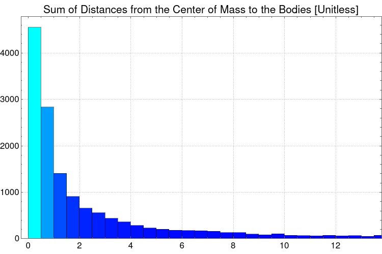
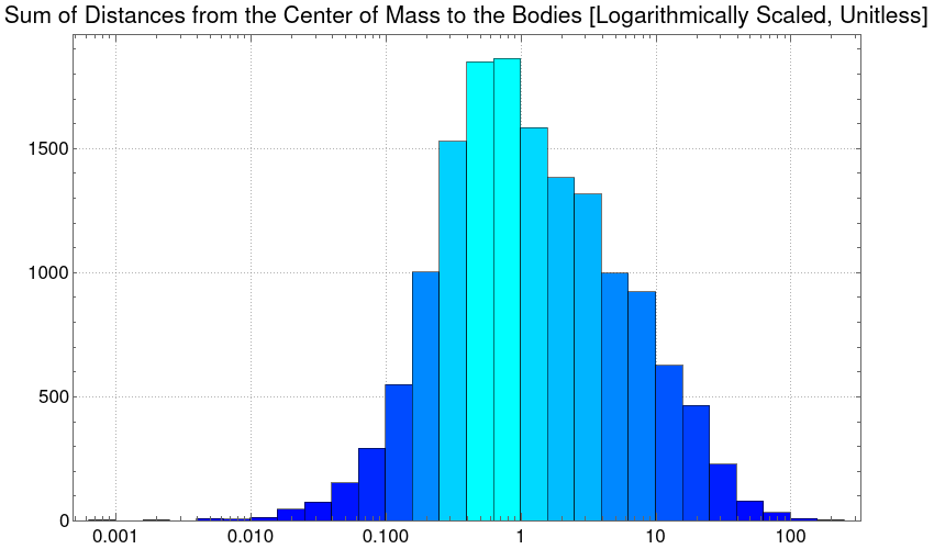
This histogram clearly shows that there's a logarithmic curve of the distances from the center of mass and the objects, in fact, a LogNormalDistribution[] distribution can be matched using FindDistribution[].
And, by plotting the histogram with a logarithmic scale, we obtain a normal distribution.
Histogram[Flatten@distancesCOM, {"Log", 20},
 PlotLabel ->
  "Sum of Distances from the Center of Mass to the Bodies \
[Logarithmically Scaled, Unitless]", LabelStyle -> {16, GrayLevel[0]},
  PlotTheme -> "Detailed",
 ColorFunction -> Function[{height}, RGBColor[0, 1*height, 1]],
 ImageSize -> {850, 500}]
One fascinating visualization is to FeatureSpacePlot all the rasterizations of the simulations. This should give us an interesting view of the bigger picture of the simulations.
rasterizeList = Rasterize[NBodyPlot[NBodySimulation["InverseSquare", #, 10]]] &/@ Normal[RandomSample[NBParametersDataset, 250]] // Quiet;

FeatureSpacePlot[rasterizeList[[1;;200]], LabelingSize -> 30, ImageSize -> {800, 800}, PlotLabel -> "Feature Space of 250 Three Body Simulations", LabelStyle -> {16, GrayLevel[0]}]
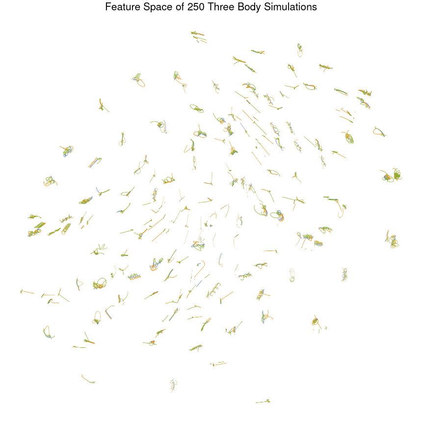
Based on this FeatureSpacePlot[], we can infer that the most caotic simulations are located in the borders, and the divergent simulations are always on the side of where is the body diverging.
Conclusion
In this project, I conclude that the applicability of algorithms such as neural networks and clustering classification is hard due to the chaotic nature of the n-body simulations, the volatility of such systems do not allow such thing as classification. Some inference could be achieved in the graphics and distributions, such as stability in lower masses, and the close center of mass from the systems.
An interesting expansion to research is to produce the same analysis on larger systems, such as a five body problem. In a more robust computer, more simulations can be done, and clearer correlations and curves should be likely to conceive.
[Optional] How to Generate the Data
For generating all the data used in this project, these cells can be executed, note that this section is an appendix, and not necessary since 5000 sample data are already included in this post notebook.
batchPath = NotebookDirectory[]

{generatedData, heuristicData, nbdpathsData, bodyData, bodiesData} = Table[{}, {5}];

NBodyHeuristics[positionsList_,maxSpace_:8] := Block[{
  emptyList = {},
  bodyA = positionsList[[1]],
  bodyB = positionsList[[2]],
  bodyC = positionsList[[3]]
},
  If[maxSpace >= bodyA[[1]] >= -maxSpace \[And] maxSpace >= bodyA[[2]] >= -maxSpace,
    emptyList = Join[emptyList, {True}],
    emptyList = Join[emptyList, {False}]
  ];
  If[maxSpace >= bodyB[[1]] >= -maxSpace \[And] maxSpace >= bodyB[[2]] >= -maxSpace,
    emptyList = Join[emptyList, {True}],
    emptyList = Join[emptyList, {False}]
  ];
  If[maxSpace >= bodyC[[1]] >= -maxSpace \[And] maxSpace >= bodyC[[2]] >= -maxSpace,
    emptyList = Join[emptyList, {True}],
    emptyList = Join[emptyList, {False}]
  ];
  Return[emptyList];
]

GenerateNBodySimulations[nsimulations_,time_] := Do[AbortProtect[
    PrintTemporary[Style["\[DoubleRightArrow]", 15, Orange], " ",
       "Generated ", Dynamic[Length[heuristicData]], " ", Style["NBodySimulations", Orange], " ",
       ProgressIndicator[Appearance -> "Percolate", ImageSize -> {60, 20}]
    ];
    bodyData = {CreateRandomPivot[], CreateRandomBody[], CreateRandomBody[]};
    generatedData = NBodySimulation["InverseSquare", bodyData, time] // Quiet;
    heuristicData = Append[heuristicData, NBodyHeuristics[generatedData[All, "Position", generatedData["SimulationTime"]]]];nbdpathsData = Append[nbdpathsData, generatedData[All, "Position", generatedData["SimulationTime"]]]];bodiesData = Append[bodiesData, bodyData];
    ClearAll[generatedData, bodyData],
    nsimulations
];

GenerateNBodySimulations[100, 10]

Export[batchPath <> "HeuristicData_" <> ToString[batchCounter] <> ".mx", heuristicData];
Export[batchPath <> "NBDPaths_" <> ToString[batchCounter] <> ".mx", nbdpathsData];
Export[batchPath <> "NBParameters_" <> ToString[batchCounter] <> ".mx", bodiesData];
{generatedData,heuristicData,nbdpathsData,bodyData,bodiesData}=Table[{},{5}];
batchCounter++;
 Attachments:


