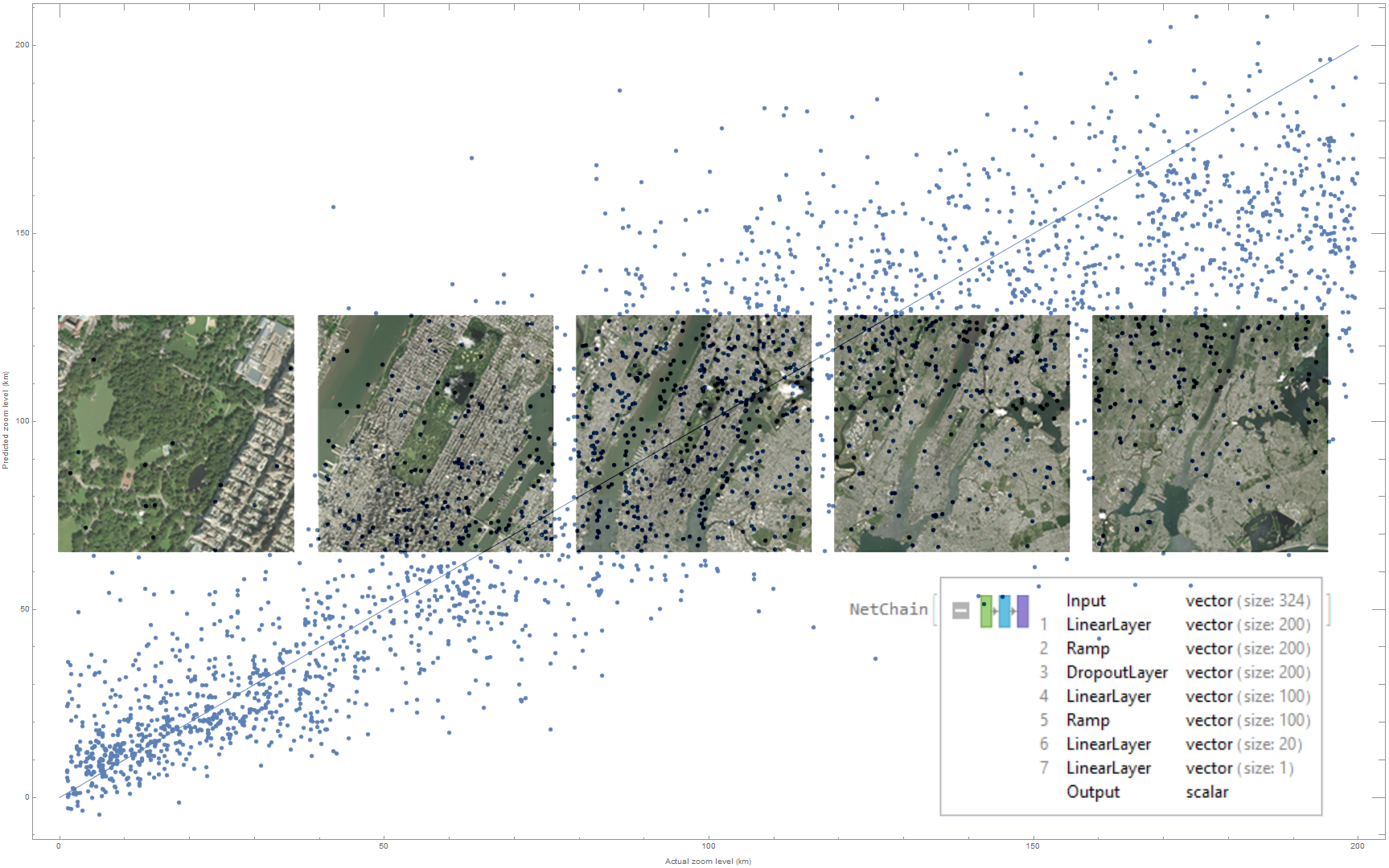
What are we trying to do?
The goal of this project is to produce an algorithm which can find the physical scale of any satellite image: the relationship between the content of the image, and the area it covers in kilometers.

This is a very challenging problem because of the characteristics of the world's terrain. At different zoom levels, it's highly self-similar, like a fractal. We need to find a method to extract useful information from these images, while also ignoring the parts which are repeated across zoom levels.
There are several ways to approach the problem. Some of the more manual methods involve trying to label image parts which only show up at certain scales. For instance, you could rely on the fact that all rooftops are generally roughly the same size, all roads have similar widths, and so on.

Those approaches all need lots of manual work, though. We attempted to solve the problem automatically, exploring ideas that might let us predict map zoom without relying on hard-coded rules.
Although we explored several approaches to this problem, the most successful solution used feature extraction to convert each image to a relatively small vector, then trained a small feed-forward neural network to predict zoom from each set of features. Although the self-similarity of each image makes more traditional CV approaches very difficult, a neural network can learn the right features to approximate the zoom very well.
Methodology
We wound up gathering several datasets of satellite images over the course of the project. The most useful one was a dataset of three thousand images of random locations in the continental United States, all taken at different zoom levels:
(* define a function to download images of a specific location and zoom *)
satelliteImage[location_, size_?NumericQ] :=
	GeoImage[
		GeoDisk[location, Quantity[size/2, "km"]],
		GeoServer -> "DigitalGlobe",
		RasterSize -> 400
	]

sampleCount = 3000;

(* Get a list of 3000 random locations in the continental US *)
randomLocations =
  RandomGeoPosition[Entity["Country", "UnitedStates"],
    sampleCount] /. GeoPosition[locs_List] :> GeoPosition /@ locs;

(* Get a list of 1000 random zoom levels, from 1 to 200 km *)
randomZooms = Table[RandomReal[{1, 200}], sampleCount];

(* create a dataset of image specifications *)
samples = MapThread[
	<|"Location" -> #1, "Zoom" -> #2|> &,
	{randomLocations, randomZooms}
] // Dataset;

(* to see the precise scripts used to download each image, download the attached notebook--they have dynamic progress indicators and checkpoint the data to disk, so they're a little complicated *)
Working on this project, the majority of the time was spent trying several different methods to extract information from images.
One attempt was visual pre-processing: running segmentation or binarization on each image before training a model or extracting some metric. Every time we did this, although the images looked really neat, the accuracy of our predictions were far worse.

All of those preprocessing methods reduce the dimensionality of the images, but it turns out that they focus on the wrong features in the process. Our network was supposed to pick up on the large patterns: rivers, landmasses, and so on. When we segmented images, the network was forced to focus on the small details we highlighted. All in all, preprocessing using traditional CV was a failure.
We also tried training a convolutional neural network from scratch on the images, which also failed. The network would, at first, immediately overfit the training set. When we reduced its size, it would fail to converge at all. Despite hours of tweaking, this method did not work either.
The next idea we had was just to throw the entire dataset into Predict[] and see what would happen. This worked shockingly well, considering how easy it was:
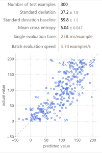
So the next question we had was: how? What was Predict[] doing behind the scenes? Doing some research, we discovered a couple starting points for our own neural network model:
Predict[] preprocesses images using WL's feature extraction functionality. This is based on the first few layers of the trained ImageIdentify convnet, combined with an autoencoder.Predict[] generally trains small feed-forward networks, without convolutional layers.
Our general approach was to replicate this setup, with several tweaks and optimizations for better performance.
Our first large improvement was a pre-processing step: image augmentation. We applied several different constant crops, translations, rotations, and reflections to each image, in order to increase the number of examples we had by a factor of 10. We then performed feature extraciton on the augmented data.
(* use the built-in augmentation functionality *)
(* note: this can't go in the network itself because we need to extract features with FeatureExtraction[] after this step *)
augmentor = ImageAugmentationLayer[
	(* Final image dimensions--from cropping *)
	{200, 200},

	(* 50% change of either reflection *)
	"ReflectionProbabilities" -> {0.5, 0.5},

	"Input" -> NetEncoder[{"Image", {400, 400}}], (* 400x400 input images *)
	"Output" -> NetDecoder["Image"] (* output an image for the feature extractor *)
]

(* each original image gets 10 augmented images generated from it *)
augmentationMultiplier = 10;

(* actually augment the image set *)
augmentedImages = Join@@Table[
	imageSet[ All, <|
		#,
		"Image" -> augmentor[#Image, NetEvaluationMode -> "Train"]
	|> &],
	augmentationMultiplier
] // RandomSample;
Our next approach was to replicate this--use FeatureExtraction[] to reduce the dimensionality of the images, and train a small, mostly-linear neural network on the result.
(* create a feature extractor trained with the first 5000 images*)
fExtractor = FeatureExtraction[augmentedImages[;; 5000, "Image"]];

(* extract features from the images *)
features = imageSet[All, <|#, "Features" -> fExtractor[#Image]|> &]
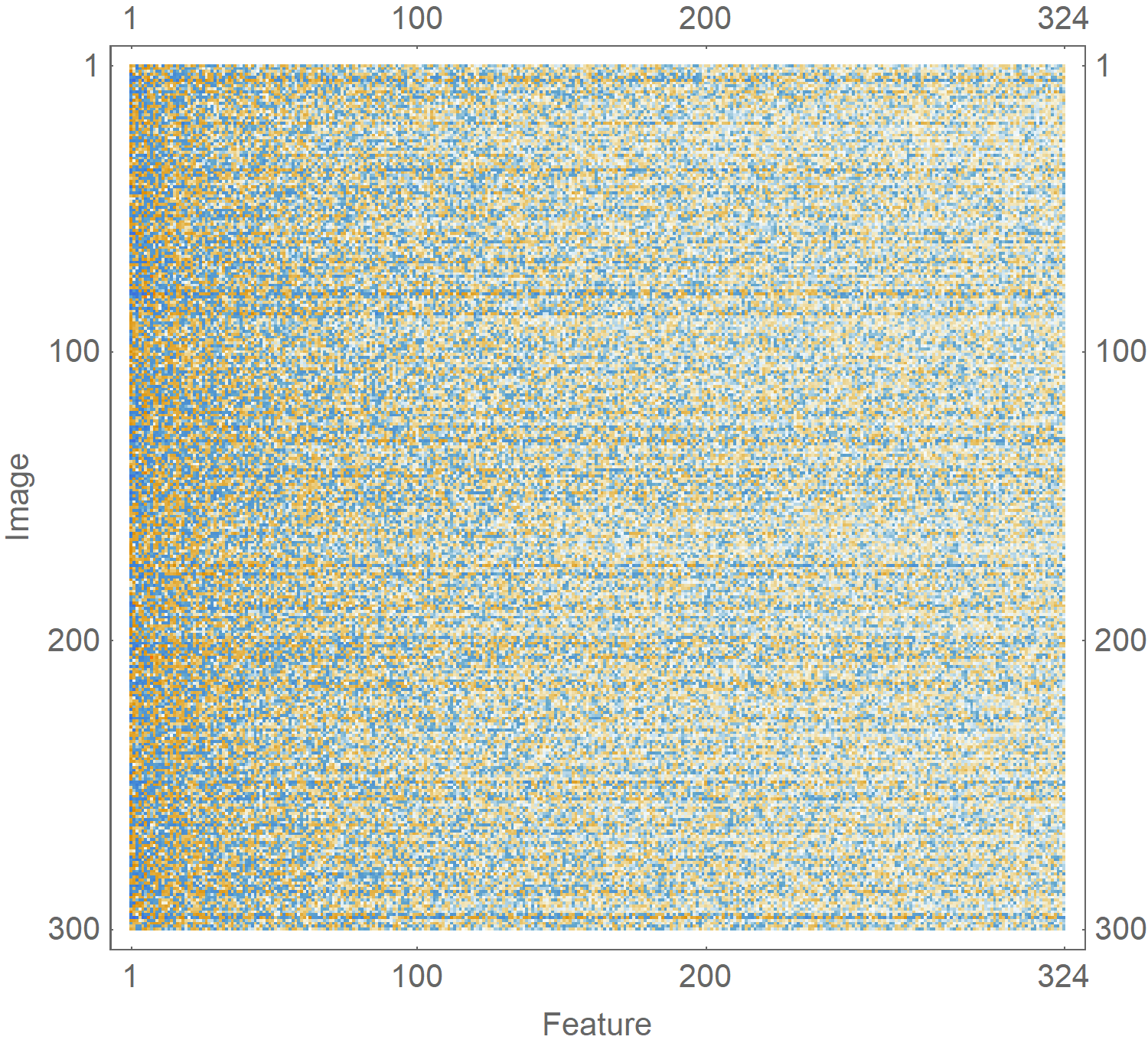
When you plot the feature vectors of a few images, you can see the variance between them is clear:
Although the network structure was fairly simple, we automated the generation of good hyperparameters. We trained hundreds of slightly-different networks, and evaluated their statistical performance. Out of many different permutations of layer count, layer size, activation function choice, training speed, and so on, we picked the ones which work best. The final network design we settled on was this:
geoNet = NetChain[
	{
		200, Ramp, DropoutLayer[0.3],
		100, Ramp,
		20,
		1
	},
	"Input" -> {324}, (* our feature vectors are 335-dimensional *)
	"Output" -> NetDecoder["Scalar"] (* decode into a single number:
	zoom in km *)
];
geoNet = NetTrain[
	geoNet,

	(* feature(Train|Test) all have the shape { {feature, ...} -> zoom, ...} *)
	featureTrain,
	ValidationSet -> featureTest,

	TargetDevice -> "GPU",
	MaxTrainingRounds -> 600,

	(* bail if loss stops decreasing *)
	TrainingStoppingCriterion -> <|"Criterion" -> "Loss", "Patience" -> 50|>
]
In the end, the general architecture of the most successful model looked like this:
+--------------------+
|                    |
|  Original dataset  |                            Generated from GeoImage[]
|                    |
+--------------------+
  |   |   |   |
  |   |   |   |
  V   V   V   V
+---------------------------+
| +---------------------------+
| | +---------------------------+
| | |                       | | |                 Generated with
| | |   Augmented dataset   | | |                 ImageAugmentationLayer[]
| | |                       | | |
+-|-|-----------------------+ | |
  +-|-------------------------+ |
    +---------------------------+
  |   |   |   |
  |   |   |   |
  V   V   V   V
 ----------------------------------------------
 ----------------------------------------------
 ------- Extracted feature vectors ------------   using FeatureExtraction[]
 ----------------------------------------------
 ----------------------------------------------
  |   |   |   |
  |   |   |   |
  V   V   V   V
 #  #  #  #  #  #  #  #  #  #  #  #  #  #  #      Small-ish neural network
 |\/|\/|\/|\/|\/|\/|\/|  /  /  /  /  /  /  /
 |/\|/\|/\|/\|/\|/\|/\|-/--/--/--/--/--/--/
 #  #  #  #  #  #  #  #
 |\/|\/|\/|  /  /  /  /
 |/\|/\|/\|-/--/--/--/
 #  #  #  #
 |-/--/--/
 |
 #                                            <-- our final prediction!
( https://textik.com/#e650301054ce435f )
Results
When we evaluated each image in our test set with this network, we got the following results:
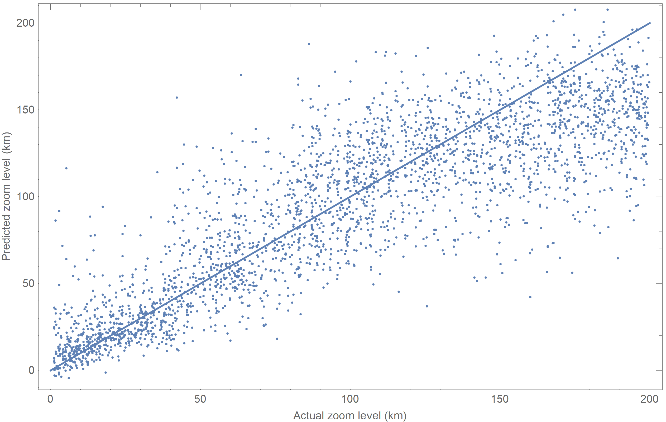
This plot shows actual zoom levels on the $x$-axis, and estimated zoom on the $y$. A reference line shows what a perfect prediction would look like. Analyzed statistically, the network had a standard deviation of 30.37 km, and an $r^2$ value of 0.732.
This network clearly "gets the gist" of the data it's presented. However, these results were not portable to different satellite image datasets. When we evaluated a separate test set, gathered from Wolfram satellite imagery, we got this result:
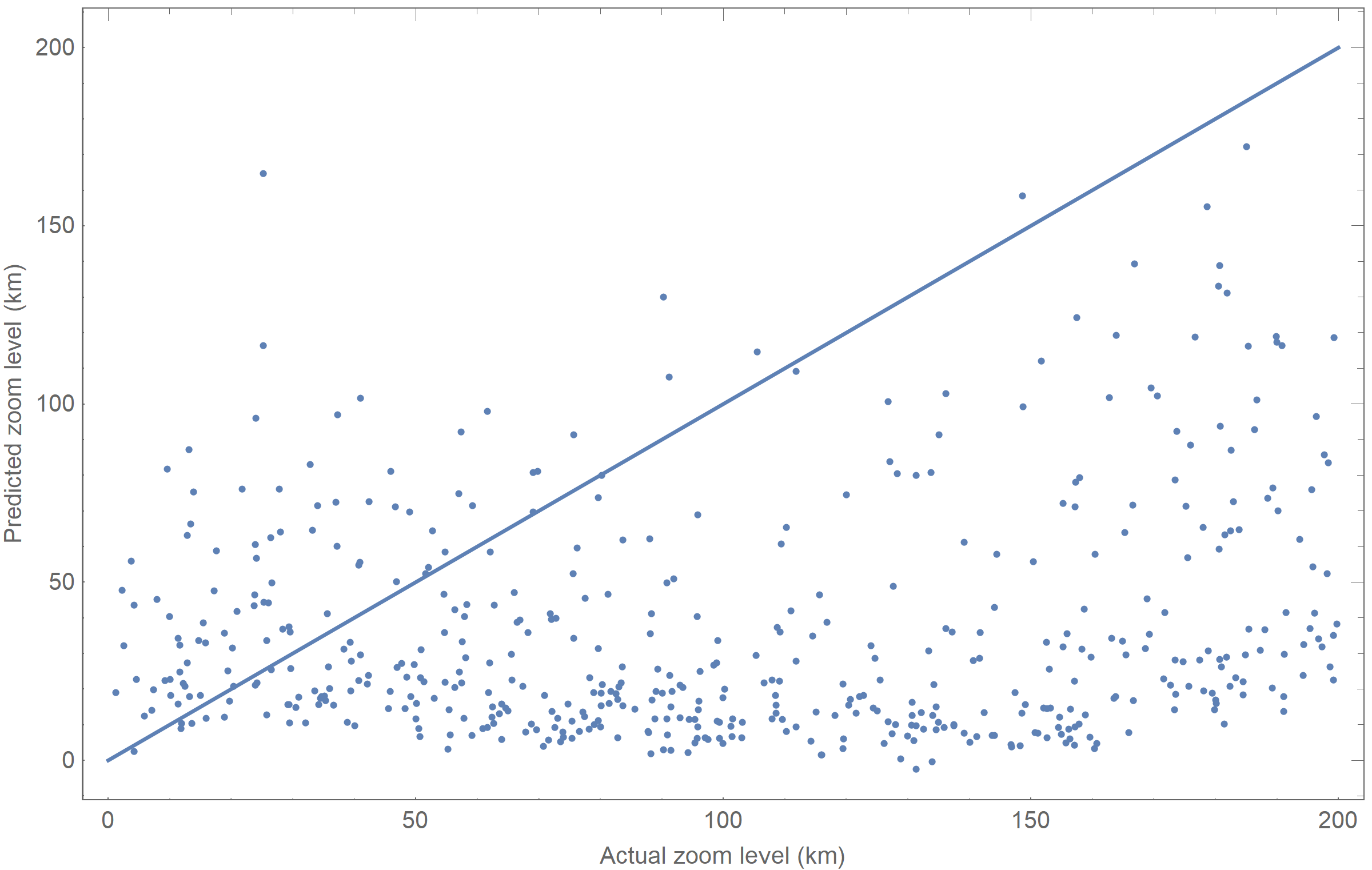
It is clear that the network is learning something specific to the DigitalGlobe dataset we used to train it. We would hesitate to call that overfitting, because it can extrapolate to locations it has never seen before, but it relies on the specific look and tone of the DigitalGlobe data. After all, the two image sets look very different:
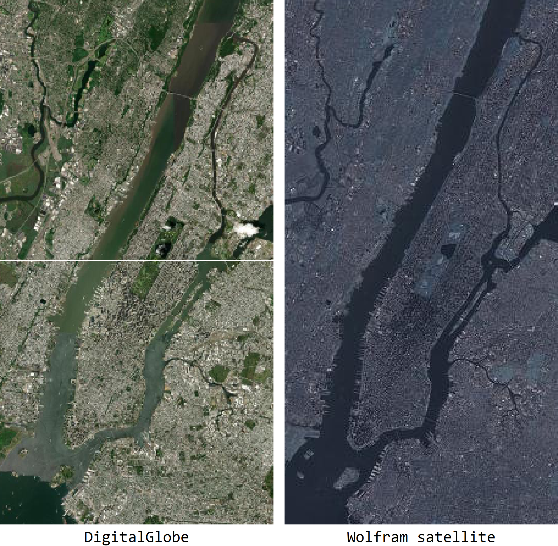
It is possible that the network is just confused by the new colors, rather than confused by the structure of the terrain in the Wolfram dataset. Either way, though, the scope of this result is limited to images similar to the satellite dataset on which it was trained.
We used another dataset of 20,000 mostly-overlapping images of Massachusetts and exploited overfitting to achieve a much more accurate (yet fragile) prediction. By managing to overfit the terrain, the model could achieve up to an $r^2$ of 0.99, but completely fell apart on any other dataset. Theoretically, you could take this brute-force approach with the entire planet, overfitting deliberately to learn the terrain. However, in our scope, we could not attempt this.
Future work
One of the larger problems with this research was gathering data. In future attempts, it would be better to gather a much larger dataset (somewhere around 50,000 images) from several different satellite providers. To stop the network from overfitting on the fine-grained style of the images, we would need to find satellite providers whose data are significantly different.
One other option is to improve the model's feature extraction layer. Right now, the FeatureExtraction function uses the first few convolutional layers of the Wolfram ImageIdentify classifier as a starting point. By training our own convolution step specific to satellite images on a much larger dataset, we might be able to get more accurate results.
Final thoughts
This research was successful in very limited scope. Future attempts at cracking this problem will have to successfully generalize to the entire globe, across several satellite image providers---a problem requiring a lot of time, and access to large computational resources, to solve.