Message Boards Message Boards

Bayesian linear regression in Mathematica

Recently I updated my Bayesian inference reporitory with a new function called BayesianLinearRegression to provide a Bayesian alternative to Mathematica's LinearModelFit. I also submitted the code for this function to the Wolfram function repository to make it easier to access, so the function can also be used with ResourceFunction["BayesianLinearRegression"].

The example notebook in the repository provides several examples of how the function can be used, some of which I will reproduce below. Please refer to the GitHub README.md file (which is displayed on the homepage of the repository) for instructions about installing the BayesianInference package. The code is in this file, in case you're interested in taking a look under the hood.

Fitting polynomials

First generate some test data:

data = RandomVariate[
  MultinormalDistribution[{{1, 0.7}, {0.7, 1}}],
  20
];
ListPlot[data]
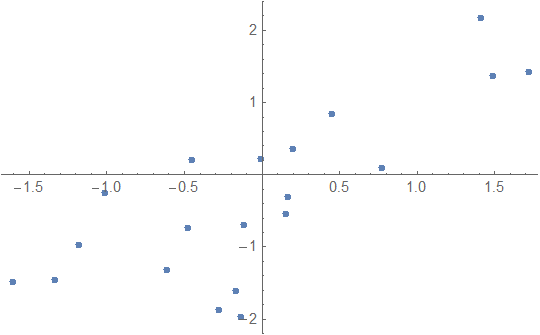
enter image description here

The usage of BayesianLinearRegression is similar to that of LinearModelFit with one significant difference: I decided that the Rule-based data specification used by Predict and NetTrain is often more convenient than the matrix input used by the Fit family, so I decided that both types of data specifications should work. The main reason for this is that BayesianLinearRegression also supports regression of vector outputs (an example of that is given in the repository example notebook), in which case the Rule-based format is often easier to understand.

When you fit a model, BayesianLinearRegression returns an Association containing all relevant information about the fit. Fit a model of the form y == a + b x + randomness where randomness is distributed as NormalDistribution[0, sigma]. Here, a, b and sigma are unknowns that need to be fitted to the data:

In[20]:= Clear[x];
model =  BayesianLinearRegression[data, {1, x}, x];

Below is a more detailed description of the information return by BayesianLinearRegression, but let's first concentrate on the main fit result, which is the posterior predictive distribution :

In[61]:= model["Posterior", "PredictiveDistribution"]

Out[61]= StudentTDistribution[-0.267818 + 0.986121 x, 
 0.726105 Sqrt[1.05016 + 0.00692863 x + 0.0635094 x^2], 
 2001/100
]

As you can see, the result is returned is an x-dependent StudentTDistribution. Visualize the predictions:

With[{
  predictiveDist = model["Posterior", "PredictiveDistribution"],
  bands = {95, 50, 5}
  },
 Show[
  Plot[
   Evaluate@InverseCDF[predictiveDist, bands/100],
   {x, -4, 4}, Filling -> {1 -> {2}, 3 -> {2}}, PlotLegends -> bands
   ],
  ListPlot[data],
  PlotRange -> All
  ]
 ]
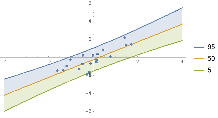
enter image description here

In the BayesianInference package on GitHub, I included a function called regressionPlot1D which makes it a bit easier to make this plot:

Show[
 regressionPlot1D[model["Posterior", "PredictiveDistribution"], {x, -4, 4}, {95, 50, 5}],
 ListPlot[data]
] 
(* same result*)

Model comparison and model mixing

Often you'll want to compare multiple models against a data set to see which one works best. For example, here is some data where it's a bit unclear if you should use a first or second order model:

data = {{-1.5`,-1.375`},{-1.34375`,-2.375`},{1.5`,0.21875`},{1.03125`,0.6875`},{-0.5`,-0.59375`},
  {-1.875`,-2.59375`},{1.625`,1.1875`},{-2.0625`,-1.875`},{1.0625`,0.5`},{-0.4375`,-0.28125`},{-0.75`,-0.75`},{2.125`,0.375`},{0.4375`,0.6875`},{-1.3125`,-0.75`},{-1.125`,-0.21875`},
  {0.625`,0.40625`},{-0.25`,0.59375`},{-1.875`,-1.625`},{-1.`,-0.8125`},{0.4375`,-0.09375`}}
ListPlot[data]
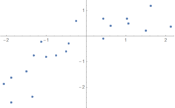
enter image description here

Fit the data with polynomials up to fourth degree; rank the log-evidences and inspect them. As you can see, the first and second order fits are almost equally likely:

In[152]:= models = AssociationMap[
   BayesianLinearRegression[Rule @@@ data, x^Range[0, #], x] &,
   Range[0, 4]
   ];
ReverseSort@models[[All, "LogEvidence"]]

Out[153]= <|1 -> -30.0072, 2 -> -30.1774, 3 -> -34.4292, 4 -> -38.7037, 0 -> -38.787|>

Show the prediction bands:

Show[
 regressionPlot1D[ models[1, "Posterior", "PredictiveDistribution"], {x, -3, 3}],
 regressionPlot1D[models[2, "Posterior", "PredictiveDistribution"], {x, -3, 3},  PlotStyle -> Dashed, PlotLegends -> None],
 ListPlot[data]
]
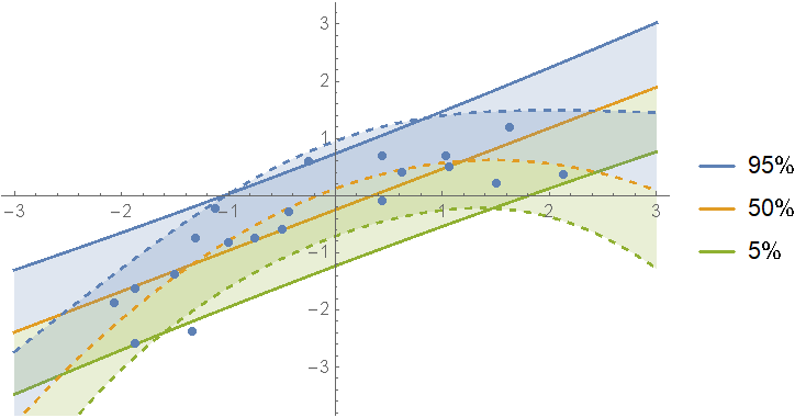
Comparison of the first (solid) and second order (dashed) prediction bands

Instead of picking just one of the models, we can define a mixture over all of them. First calculate the weights for each fit:

In[94]:= weights = Normalize[
   (* subtract the max to reduce rounding error *)
   Exp[models[[All, "LogEvidence"]] - Max[models[[All, "LogEvidence"]]]],
   Total
   ];
ReverseSort[weights]

Out[95]= <|1 -> 0.516002, 2 -> 0.47702, 3 -> 0.0068122, 4 -> 0.0000982526, 
 0 -> 0.0000667854|>

Define a mixture of posterior predictive distributions and show the predictions:

In[96]:= mixDist = MixtureDistribution[
   Values[weights],
   Values@models[[All, "Posterior", "PredictiveDistribution"]]
   ];
Show[
 regressionPlot1D[mixDist, {x, -3, 3}],
 ListPlot[data]
 ]
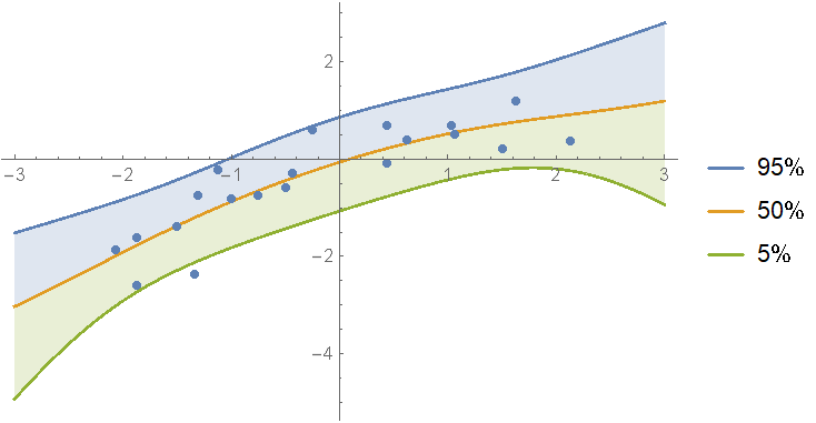
Prediction bands of a mixture of polynomial models up to degree 4

As you can see, if one model is not clearly the best, you can just split the difference between them.

Another interesting thing you can do with BayesianLinearRegression is Bayesian updating. Basically, this means that if you've fitted some data in the past and are now finding new data, you can incorporate the new data by updating your fit without having to re-fit all of the data (old and new) in one go. An example of this is given in the example code notebook on GitHub (in the section about the "PriorParameters" options of the function).

Detailed explanation about the returned values

BayesianLinearRegression returns an Association with the following keys:

Keys[model]

Out[21]= {"LogEvidence", "PriorParameters", "PosteriorParameters", "Posterior", "Prior", "Basis", "IndependentVariables"}
  • "LogEvidence": In a Bayesian setting, the evidence (also called marginal likelihood) measures how well the model fits the data (with a higher evidence indicating a better fit). The evidence has the virtue that it naturally penalizes models for their complexity and therefore does not suffer from over-fitting in the way that measures like the sum-of-squares or likelihood do.
  • "Basis", "IndependentVariables": Simply the basis functions and independent variable specified by the user.
  • "Posterior", "Prior": These two keys each hold an association with 4 distributions:
  1. "PredictiveDistribution": A distribution that depends on the independent variables (x in the example above). By filling in a value for x, you get a distribution that tells you where you could expect to find future y values. This distribution accounts for all relevant uncertainties in the model: model variance caused by the term randomness; uncertainty in the values of a and b; and uncertainty in sigma.
  2. "UnderlyingValueDistribution": Similar to "PredictiveDistribution", but this distribution give the possible values of a + b x without the randomness error term.
  3. "RegressionCoefficientDistribution": The join distribution over a and b.
  4. "ErrorDistribution": The distribution of the variance sigma^2.
  • "PriorParameters", "PosteriorParameters": These parameters are not immediately important most of the time, but they contain all of the relevant information about the fit.

Sources

The formulas underlying BayesianLinearRegression are based mainly on the following Wikipedia articles. The names of the hyper parameters returned by the function are based on the article about multivariate linear regression.

POSTED BY: Sjoerd Smit
19 Replies

enter image description here - Congratulations! This post is now featured in our Staff Pick column as distinguished by a badge on your profile of a Featured Contributor! Thank you, keep it coming, and consider contributing your work to the The Notebook Archive!

POSTED BY: EDITORIAL BOARD
Posted 5 years ago

Hi Sjoerd

This is all really interesting material, thanks for posting it. Working through the BayesianInference examples, I ran into a problem with "Logistic classification with multi dimensional input and multiple classes" examples, the defineInferenceProblem evaluation shows $Failed for "GeneratingDistribution". I tried to figure out what might be amiss but without success - any suggestions?

I am using the package updated in July and the corresponding examples notebook running on version 12.0

-Steve

POSTED BY: Steve Walker

Hi Steve,

Yes, I can see what you ran into. I will admit that that particular example isn't worked out all that well. I more or less worked that out for myself and plonked it in for future reference. I assume you're referring to the fact that the tooltip of the inferenceObject shows the "GeneratingDistribution" key as $Failed? From what I can tell, that's just a bug in the code that generates the tooltip: if you evaluate obj["GeneratingDistribution"] it should still return the ProbabilityDistribution that was used to in the construction of the object. I'll try and patch it out in the next push to master.

It's continuing work in progress, though I my time and attention span to work on it is not super consistent. Glad to hear that you're giving it a try, though!

POSTED BY: Sjoerd Smit
Posted 5 years ago

Hi Sjoerd

I was actually working backwards from errors thrown by parallelNestedSampling (CholeskyDecomposition error messages) and saw that there seemed to be an issue with the generating distribution from the tooltip message of the inference object. I'd looked at the distribution and couldn't see anything wrong with it (although I did wonder how the various symbols would be resolved by the sampling function), I had a quick look at the source code but didn't get anywhere (there's a lot of code).

In any case I've been finding the examples you've provided very helpful in trying to gain a better understanding of the analysis reasoning. Look forward to the next update once you've had a chance to work on it

-Steve

POSTED BY: Steve Walker

Yes, I saw those errors as well. I don't actually know where they come from; probably some part of the internal MCMC sampler I'm using. It may be a fairly harmless thing, but I don't really know to be honest. The thing with MCMC and related methods is that things hardly ever work right out of the box without tweaking some options and settings. If you let the sampler run for a while (a couple of minutes or so) it should return a result.

POSTED BY: Sjoerd Smit

Sjoerd,

Very happy to have stumbled across this as it seems to be the basis for exactly what I needed. I am wondering if it is possible to do this with multivariate polynomial regression, i.e. would something along the following lines work:

BayesianLinearRegression[data,{1,x1,x2,x1^2,x1*x2,x2^2},{x1,x2}]

Hi Daniel, Yes, that should be not problem at all. data should be either an n by 3 matrix or a list of rules of the form {{x11, x21} -> y1, ... }. From there it should work without issue, though you may need to re-scale the data if your xi or yi are very large or very small.

Oh, and before I forget: the function is now also available as a ResourceFunction, so you don't need to install the Github package if you don't want to. Just use ResourceFunction["BayesianLinearRegression"] instead of BayesianLinearRegression.

POSTED BY: Sjoerd Smit

Thanks for such a prompt reply, I look forward to giving it a try now.

Hello Sjoerd, I am excited to find your post telling that you have developed "Bayesian Linear Regression," which I was finding. Most attractive to me is that you don't have to specify prior distribution. My question is

  1. what is the 4 distributions associated with keys "Posterior" or "Prior"?
  2. can you add Weibull distribution, if not currently included?

Thank you in advance. - Toshi

POSTED BY: Toshiyuki Meshii

Are the values for the RegressionCoefficientDistribution approximate based on some form of sampling or are they supposed to be exact? If approximate, is there anyway to increase the accuracy? If exact, then either you (unlikely) or me (likely) is doing something wrong. My numbers on a toy problem are slightly different, which would be explicable if you are sampling.

POSTED BY: Seth Chandler

Hi Toshi,

The default prior distribution used is very non-informative, so normally you don't need to worry about it much except when you do want to use an informative prior. The model uses a conjugate prior (because that allows closed-form solutions) that is explained on the two Wikipedia pages I linked:

For an example of specifying the prior, please look at "PriorParameters" section (under Options) on the documentation page of my resource function:

https://resources.wolframcloud.com/FunctionRepository/resources/BayesianLinearRegression

As for including a Weibull distrbution: is there a conjugate prior for that? If not, then the current function cannot use it. The current function uses these specific distributions because there exists conjugate priors for them. I don't think there's many other choices for which nice closed-form solutions like this.

Best regards, Sjoerd

POSTED BY: Sjoerd Smit

Hi Seth,

The regression coefficient distribution should be the exact distribution, but with one caveat: the distribution of the variance parameter is only given as a marginal; not as a full multivariate distribution over all parameters together. So you only get two marginals: one over the variance and one over all the other parameters. This is because there's unfortunately no good way to represent the full multivariate PDF in the language right now. It shouldn't be too difficult to generate the full PDF from the "PosteriorParameters" vector, though, since it is just the product of a multinormal and a gamma distribution. On the documentation page of this function I give an example of such a distribution in the Applications section:

https://resources.wolframcloud.com/FunctionRepository/resources/ConditionalProductDistribution

Of course, there's also always a possibility that I made a typo in one of the formula's somewhere. I did a lot of spot-checks to weed out mistakes, but in the end the code could probably do with some external proofreading to be 100% sure.

POSTED BY: Sjoerd Smit

Attached is a notebook showing the MultivariateTDistribution for the distribution of the regression coefficients that I get out of LinearModelFit and the ones obtained from BayesianLinearRegression. I am leaning to the theory that there is nothing wrong with either my notebook or your code and that the problem is in my failure to understand Bayesian Linear Regression fully. But any enlightenment you could provide would be appreciated.

Attachments:
POSTED BY: Seth Chandler

Ah, I see. Yes, in both cases you get a T-distribution, but if you derive it from the point-estimate made with LinearModelFit (which is a frequentist method), it means something different, which is why the two results aren't identical even if they look very similar. For one, the T-distribution returned by the Bayesian method is influenced by the prior you set (which, by default, is quite uninformative but it doesn't have to be so) while in the frequentist method there is no prior at all (though sometimes there are regularizers, which serve a similar purpose). If memory serves me right, the frequentist T-distribution is the sampling distribution of the parameters over a long run of (imagined) datasets sampled from the currently estimated model while the Bayesian T-distribution is the distribution of the knowledge of the model parameters conditional on the current dataset.

A more important difference is the method for generating predictions from the fit. You may note that the lmf["SinglePredictionBands"] and lmf["MeanPredictionBands"] are different from the Bayesian bands calculated from model["Posterior", "PredictiveDistribution"] and model["Posterior", "UnderlyingValueDistribution"] because those distributions generate credible intervals and not confidence intervals. Concretely, the Bayesian bands are typically narrower because the information in the data is used more efficiently (that's a very broad simplification, of course).

I feel like this may not really do much justice to the differences in the results and in the end there's no denying that the formulas end up looking quite similar for linear models like these. The interpretation of the results is different, though, with the Bayesian results usually being closer to how people tend to intuitively interpret statistical results. If you're interested, I feel like it would be more beneficial to have a direct chat about this sometime to avoid having to go through the whole frequentist vs Bayesian discussion here.

POSTED BY: Sjoerd Smit

Hello Sjoerd Thank you for your reply. I do not know and am finding that for Weibull distribution. Weibull distribution is an important model expressing probability of brittle fracture of metals. I will appreciate your idea of Rule based data learning. Best regards, - Toshi

POSTED BY: Toshiyuki Meshii

Hi Toshi,

No problem. I just saw that the Wikipedia article about conjugate priors does mention Weibull distributions, so you might be able to implement them easily yourself. I'm not entirely certain, though, how this distribution is meant to be used in linear regression.

POSTED BY: Sjoerd Smit

Dear Sjoerd,

I have a time series of water temperature between 2019-2020 with a 15-minute interval for SKOKOMISH river, in Mason County, United States. Please see the enclosed file.

Do you have any idea for modeling this data for the very shortly (15 min or hourly) prediction process? Look forward to hearing your response.

Regards, Ghorbani

Attachments:
POSTED BY: M.A. Ghorbani

Dear Ghorbani,

It's difficult to say what would be a good model for this. There's a clear trend that can probably be fitted by a deterministic model. I'm not quite sure what you would do with the residuals after that. Presumably some model that works well for weather phenomena in general since I expect the weather to be the main driver for those temperature fluctuations. Maybe an ARMAProcess or something like that? I'm no expert on weather or climate, so I don't know what would be appropriate, to be honest.

POSTED BY: Sjoerd Smit
Posted 4 years ago

ARMA or ARIMA would be common choices for this type of time series data, I was looking at a similar dataset related to river bed depth and tried numerous approaches (e.g. RNN, an empirical physics based predictor using MCMC to fit parameters). If you're interested in a Bayesian approach to time series predictions then Bayesian structured time series is one possibility. The Inferring causal impact using Bayesian structural time-series models paper looks like a lot of work to implement but there is a R package (bsts) available (I haven't tried using it though) discussed in this article Sorry ARIMA but I'm going Bayesian. Without trying it I don't know whether it would OK through ExternalEvaluate or maybe through RLink.

POSTED BY: Steve Walker
Reply to this discussion
Community posts can be styled and formatted using the Markdown syntax.
Reply Preview
Attachments
Remove
or Discard

Group Abstract Group Abstract