This can actually be solved analytically. Consider the following. Your equation
x^y==y^x && x!=y
can actually be rewritten as
x^(1/x)==y^(1/y) && x!=y
So if we now solve equations
{x^(1/x)==t, y^(1/y)==t, x!=y}
as finding functions x(t) and y(t), we will parametrize your curve. For this let's that equation
Reduce[x^(1/x) == t && x > 0 && t > 0, x]
does have a beautiful simple solution
(t == 1 && x == 1) ||
(0 < t < 1 && x == E^-ProductLog[-Log[t]]) ||
(1 < t <= E^(1/E) && (
x == E^-ProductLog[-1, -Log[t]] ||
x == E^-ProductLog[-Log[t]]))
The same solution would go for y(t). There are two domains listed here:
0 < t < 1||1 < t <= E^(1/E)
and two functions:
E^-ProductLog[-Log[t]])||E^-ProductLog[-1, -Log[t]]
So it is obvious to avoid trivial parametric curve
x[t]==y[t]
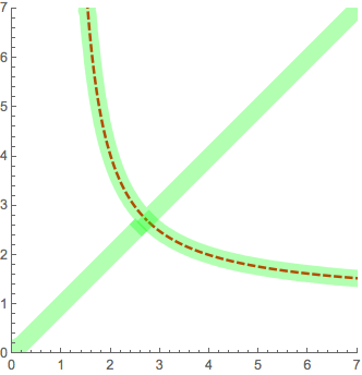
We need to choose different functions for x(t) and y(t) in the same domain. You can see how exactly overlaps the numerical plot (green, thick) with analytic formula (red, dashed):
Show[
ParametricPlot[{
{E^-ProductLog[-Log[t]], E^-ProductLog[-1, -Log[t]]},
{E^-ProductLog[-1, -Log[t]], E^-ProductLog[-Log[t]]}},
{t, 0, E^(1/E)}, PlotRange -> {{0, 7}, {0, 7}}, PlotStyle -> Directive[Thick, Dashed, Red]],
ContourPlot[x^y == y^x, {x, 0, 10}, {y, 0, 10},
ContourStyle -> Directive[Green, Thickness[.05], Opacity[.3]]]
]
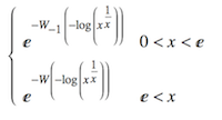
From this it is obvious to deduce the final solution:
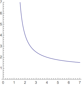
sol[x_] := Piecewise[{
{E^-ProductLog[-1, -Log[x^(1/x)]], 0 < x < E},
{E^-ProductLog[-Log[x^(1/x)]], E < x}}];
sol[x] // TraditionalForm
Plot[sol[x], {x, 0, 7}, AspectRatio -> Automatic, PlotRange -> {0, 7}]