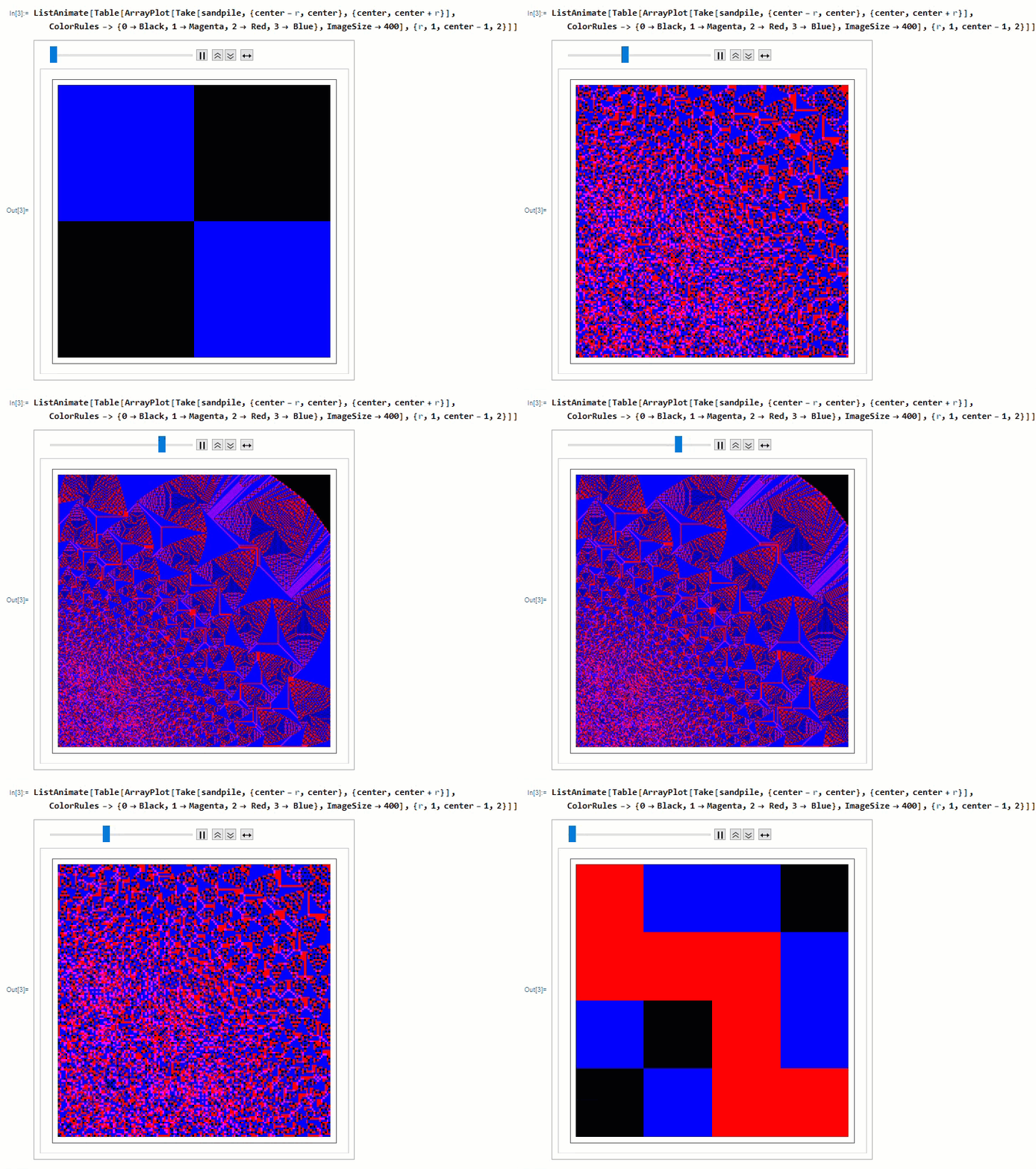
Abelian Sandpile Model

We call this Mathematica function to retrieve some background information from Wiki page: WikipediaData["Abelian sandpile model"]

The Abelian sandpile model, also known as the Bak[Dash]Tang[Dash]Wiesenfeld model, was the first discovered example of a dynamical system displaying self-organized criticality. It was introduced by Per Bak, Chao Tang and Kurt Wiesenfeld in a 1987 paper.The model is a cellular automaton.

Also in NKS there is discussion about self-organized criticality and some simple demo codes in Mathematica. You may also find this Numberhile video on this topic interesting, typically it talks about where "Abelian" comes from based on group theory point of view.

I found a GitHub repo with a nice implementation of the model in C++ and it works quite well for large number ( ~ 1 million initial sand particles at origin). I think this can be a good example to show how to use LTemplate package to call this C++ package from Mathematica if you do not want to start from scratch using the basic LibraryLink C API's.

Implementation

Follow this link to install LTemplate package and refer to the document page coming with this package to find the basic example and some type conversion information (well, not like Mathematica you need to specify the type by yourself). In particular we need mma::IntMatrixRef as return type and to transfer a 2D array back to Mathematica. Meanwhile, we also need ra = mma::makeMatrix<mint> (ra stands for raw array) to store the grid information during computation. This ra also replaces the double pointer in the original code to handle the array for plot later. Here is the code

#include <LTemplate.h>
#include <numeric>
#include <iomanip>


class sandpile {
public:

    const int dx[4] = { 1,0,-1,0 };
    const int dy[4] = { 0,1,0,-1 };
    const int N_size = 781; 
    const int N_size2 = 390;

    struct L_coord
    {
       unsigned int x;
       unsigned int y;
    };


    mma::IntMatrixRef CreateSandpile(int n ) {

        auto ra = mma::makeMatrix<mint>(N_size,N_size);
        std::fill(ra.begin(),ra.end(),0);
       bool** V_sites = new bool*[N_size];                    
       bool** Move_ = new bool*[N_size];                      
       unsigned int** Odometer = new unsigned int*[N_size];

       for (int k = 0; k < N_size; k++)
       {
         V_sites[k] = new bool[N_size];
         Odometer[k] = new unsigned int[N_size];
         Move_[k] = new bool[N_size];

         for (int i = 0; i<N_size; i++)
         {
          Move_[k][i] = false; V_sites[k][i] = false;
         }
       }

       L_coord* walking_ = new L_coord[N_size*N_size];        
       V_sites[N_size2][N_size2] = true;
       Move_[N_size2][N_size2] = true;
       ra(N_size2,N_size2) = n;
       walking_[0].x = N_size2;
       walking_[0].y = N_size2;  
       unsigned int x = 0, y = 0;
       int top_ = 0;
       unsigned int lx = 0, ly = 0;
       unsigned int d = 0; 
       unsigned int max_of_top = 0;
       unsigned long N_of_Moves = 0;

       while (top_ >= 0)
       {
         N_of_Moves += 1;
         if (max_of_top < top_) { max_of_top = top_; }

         x = walking_[top_].x;  y = walking_[top_].y;

         top_--; Move_[x][y] = false;

         d = (ra(x,y) >> 2);
         ra(x,y) = ra(x,y) - (d << 2);

         for (int k = 0; k < 4; k++)
         {
          lx = x + dx[k];
          ly = y + dy[k];

          V_sites[lx][ly] = true;
          ra(lx,ly) += d;
          if (Move_[lx][ly] == false && ra(lx,ly) >= 4)
          {
              walking_[++top_].x = lx; 
              walking_[top_].y = ly; 
              Move_[lx][ly] = true;
          }
         }
       }

        for (int k = 0; k<N_size; k++)
       {
         delete[] V_sites[k]; delete[] Odometer[k]; delete[] Move_[k];
       }
       delete[] V_sites; delete[] Odometer; delete[] Move_; delete[] walking_;
            return ra;
    }
};

I keep most part intact, only made several essential modification according to the document of LTemplate:

• Include LTemplate head file
• Create a class called sandpile which wraps around the CreateSandpile function to be imported
• Return mma::IntMatrixRef object instead of Clock object used to print computation time cost

Compile and Load

In a Mathematica notebook, I run the following lines. First I need to load the package

<< LTemplate`
SetDirectory[NotebookDirectory[]] (*put sandpile.h in the same directory as the working nb*)

we need to tell Mathematica which class to load and to pick the right member function at the same time

template =LClass["sandpile",{
    LFun["CreateSandpile", {Integer}, {Integer, 2}]
    }];

If our compiler is set up correctly, with verbose log, we should compile the class to dll just like in VS developer command or xcode or some clang/gcc environment on Linux.

CompileTemplate[template,
"ShellCommandFunction" -> Print, "ShellOutputFunction"->Print
]

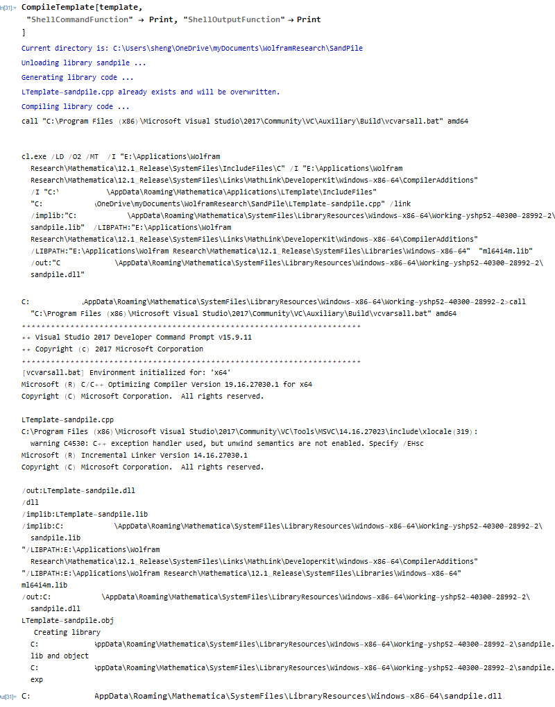
The last line is the dll in the $UserBaseDirectory. Then we can load the dll with

LoadTemplate[template]

Import the class

sp = Make["sandpile"]

and call the member function:

sp@"CreateSandpile"[100]

I omitted one ArrayTrim function in C++ code to simplify the process. We actually need it to trim margins with all zeros in a row or column. I choose to implement it quickly in Mathematica with much shorter lines than the c++ version, even though we might transferred many null points back to kernel wasted. Nevertheless,

cleanRow[arr_] := DeleteCases[arr, _?(Total@# == 0 &)]

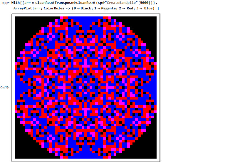
For small set, the

With[{arr = cleanRow@Transpose@cleanRow@(sp@"CreateSandpile"[5000])}, 
 ArrayPlot[arr, ColorRules -> {0 -> Black, 1 -> Magenta, 2 -> Red, 3 -> Blue}]]

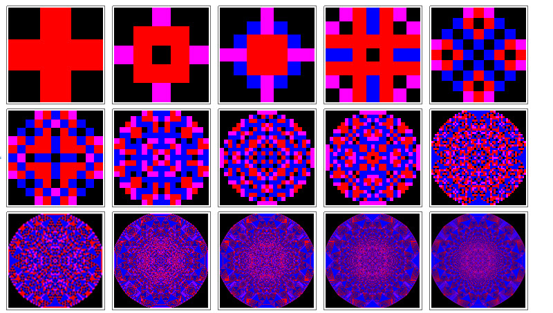
Growing complexity

Style[Grid[Partition[Map[With[{arr=cleanRow@Transpose@cleanRow@(sp@"CreateSandpile"[#])},
ArrayPlot[arr,ColorRules->{0->Black,1->Magenta,2-> Red,3-> Blue}]]&,
{10,20,50,80,100,200,500,800,1000,5000,10000,50000,100000,200000,500000}],5]],
ImageSizeMultipliers->0.4]

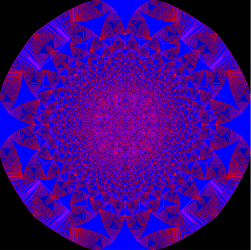
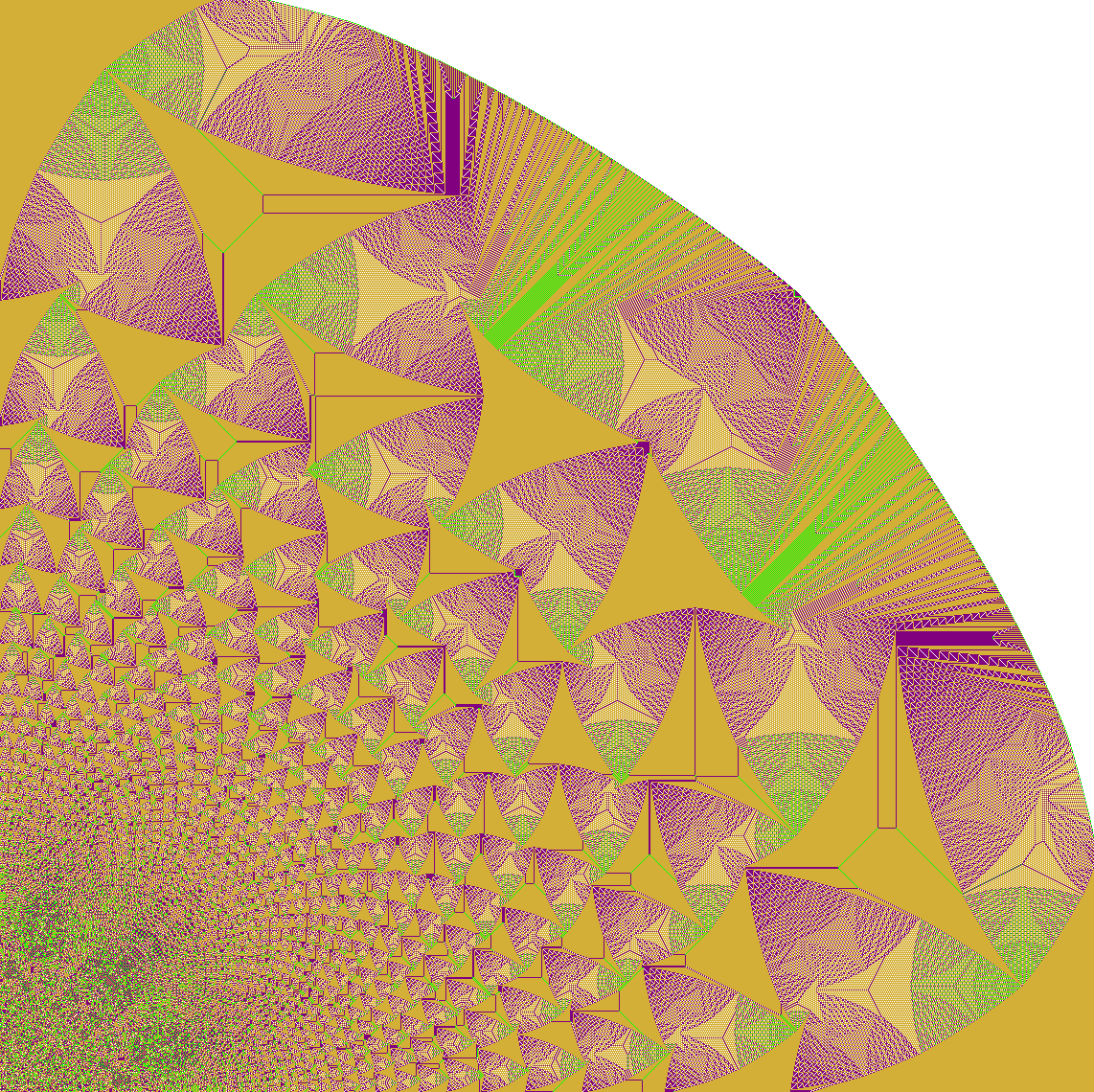
I tested the code on 10 million initial points and no problem at all to display it nicely with ArrayPlot. The animation at the beginning is only shows a quarter of the whole graph due to symmetry. The color scheme is the same as the original post.

• 1 Million particles at center at t-zero

  With[{arr = cleanRow@Transpose@cleanRow@(sp2@"CreateSandpile"[1000000])}, 
  ArrayPlot[arr,ColorRules -> {0 -> Black, 1 -> Magenta, 2 -> Red, 3 -> Blue}]]
  

• 10 Million particles at center at t-zero (only show quarter) and the result is attached in csv format.

  ImageCrop@
   Colorize[sp1@"CreateSandpile"[10000000], 
    ColorRules -> {0 -> White, 1 -> Green, 2 -> Purple, 
      3 -> RGBColor["#D4AF37"]}]
  

Summary

• Use LibraryLink based package LTemplate to call a C++ function with one integer input and 2D integer output.
• Demonstrate how to pass 2D array in C++ back to Mathematica
• Use ArrayPlot to visualize tensor computed in C++ environment
• Safely wrap Manipulate or ListAnimate around external library function
• Mathematica implementation can also be found here
• Analytic research on this topic's complexity

Attachments:

sandpile10M.csv