Introduction
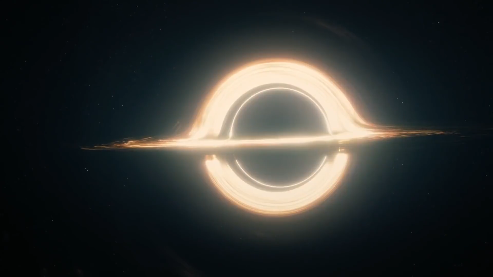
One of the most thrilling parts in Nolan's movie "Interstellar" is the black hole Gargantua and its accretion disk. Its weird shape has surely attracted lots of attention. But do black holes and their accretion disks actually look like that? Not exactly.
In the paper "Gravitational lensing by spinning black holes in astrophysics, and in the movie Interstellar", the authors say that in the movie, redshift and blueshift, as well as the intensity difference is ignored to prevent confusion to the audience. So, although the outline of the accretion disk in "Interstellar" is accurate, the color and the intensity are not. Furthermore, even in the paper, effects brought by the time delay in the propagation of light are ignored, and the influence of gravity lensing on light intensity is simplified.
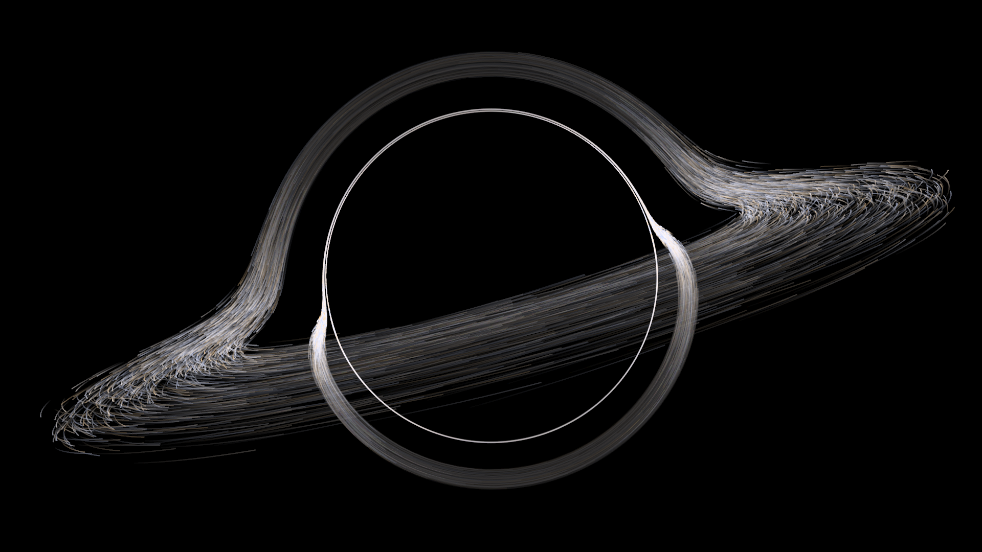
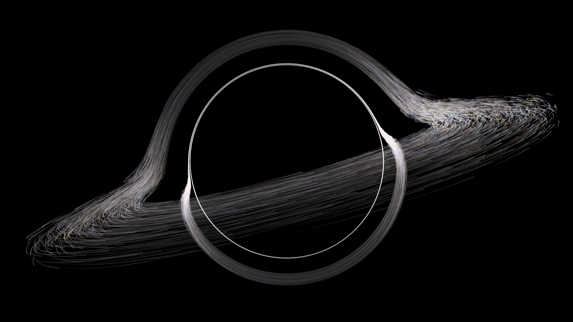
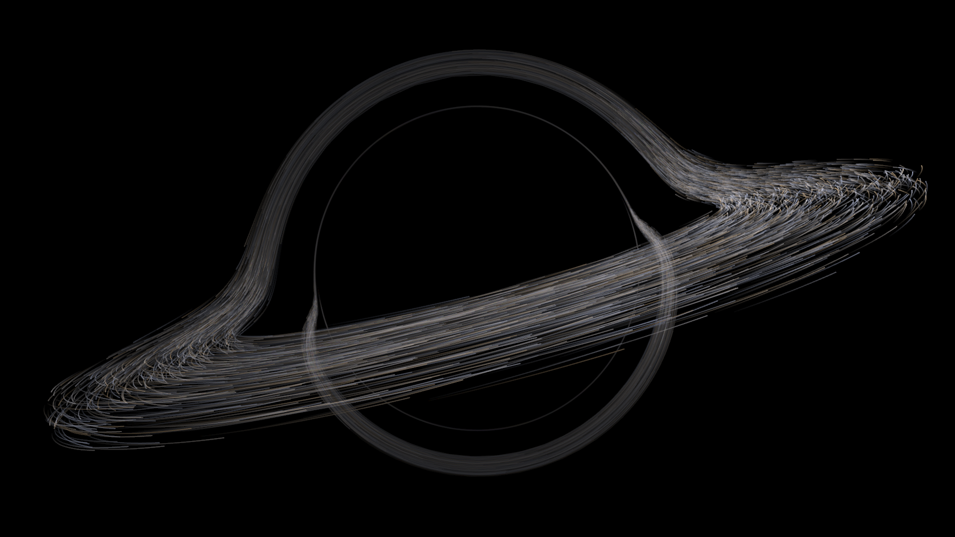
Though I cannot easily render a spinning black hole (Kerr black hole), what I can do is try to render an accretion disk around a Schwarzschild black hole, and as physically correct as possible. The result would be something like this (observer static at 6 times the Schwarzschild radius):

I strongly recommend you to see the videos at Bilibili or Youtube (Both have English subtitles) first to have a first impression, and it would be the best if you can click the vote up button XD. After that, If you would like to know more about the Mathematica realization and physical principles behind the scene, please continue.
A disclaimer first: I know nothing about accretion disk physics, so the property of accretion disks are set arbitrarily. Furthermore, actual accretion disks are actually blazingly bright, and you would be blind instantly if you are looking at it from a short distance, so I have to make some modifications.
Analytics
Physics Perspective
First, we need to analyze this problem from the physics perspective, get to know about the problems we should consider. For observers, the intensity of light is determined by how much photons reached their eye in a certain angle range, and the color is determined by the spectrum of the light. However, the orientation, spectrum, and intensity of light beams can be influenced by the observer's movement, so we have to consider that. Naturally, the next question should be, where the light comes? Well, all the light must have come from some light-emitting materials, so we have to consider the light-emitting materials' property and movement. But the light should travel for some time and distance before reaching the observer's eye. This process involves tracing the light from the emitter to the observer to determine the direction of light the observer perceived, as well as how much portion of light can reach the observer's eyes. Till now, we have already listed out all effects, from the emission to the perception, which could influence our view, so I believe this rendering is "physically accurate".
Programming Perspective
But view from the programming perspective, the zeroth problem should be how lights travel around a black hole: we need the light path to calculate all other effects. Then, based on the light path, we can directly compute the equivalent of "brighter when closer" rule, as well as the time delay between light emission and observation. If combined with the movement of the light-emitting materials and the observer, we can compute the redshift and the blueshift.
Details, Theory, Coding and Results
Now let's assume that we are stationary observers viewing from 6 times the Schwarzchild radius.
Ray Tracing
The first problem to solve is tracing the light beam. Light bends around black holes following the geodesics, and the most apparent consequence of this would be that the accretion disk we see would not be on a plane, but rather curved and bent. Fortunately for us, because Schwartzchild black holes are spherically symmetric, we can reduce the problem to 2D. The parametric equation of geodesics around a Schwarzschild black hole can be derived as follows:
$$ \left{ \begin{aligned} t''(\lambda)&=\frac{Rs r' t'}{Rs r-r^2}\ r''(\lambda)&=\frac{-Rs r^2 r'^2-2r^3\theta'^2(Rs-r)^2+Rs(Rs-r)^2t'^2}{2r^3(R_s-r)}\ \theta''(\lambda)&=-\frac{2r'\theta'}{r} \end{aligned} \right. $$
Where $\lambda$ is the ray parameter.
Now we construct a set of light which originates from the observer, and trace them backward:
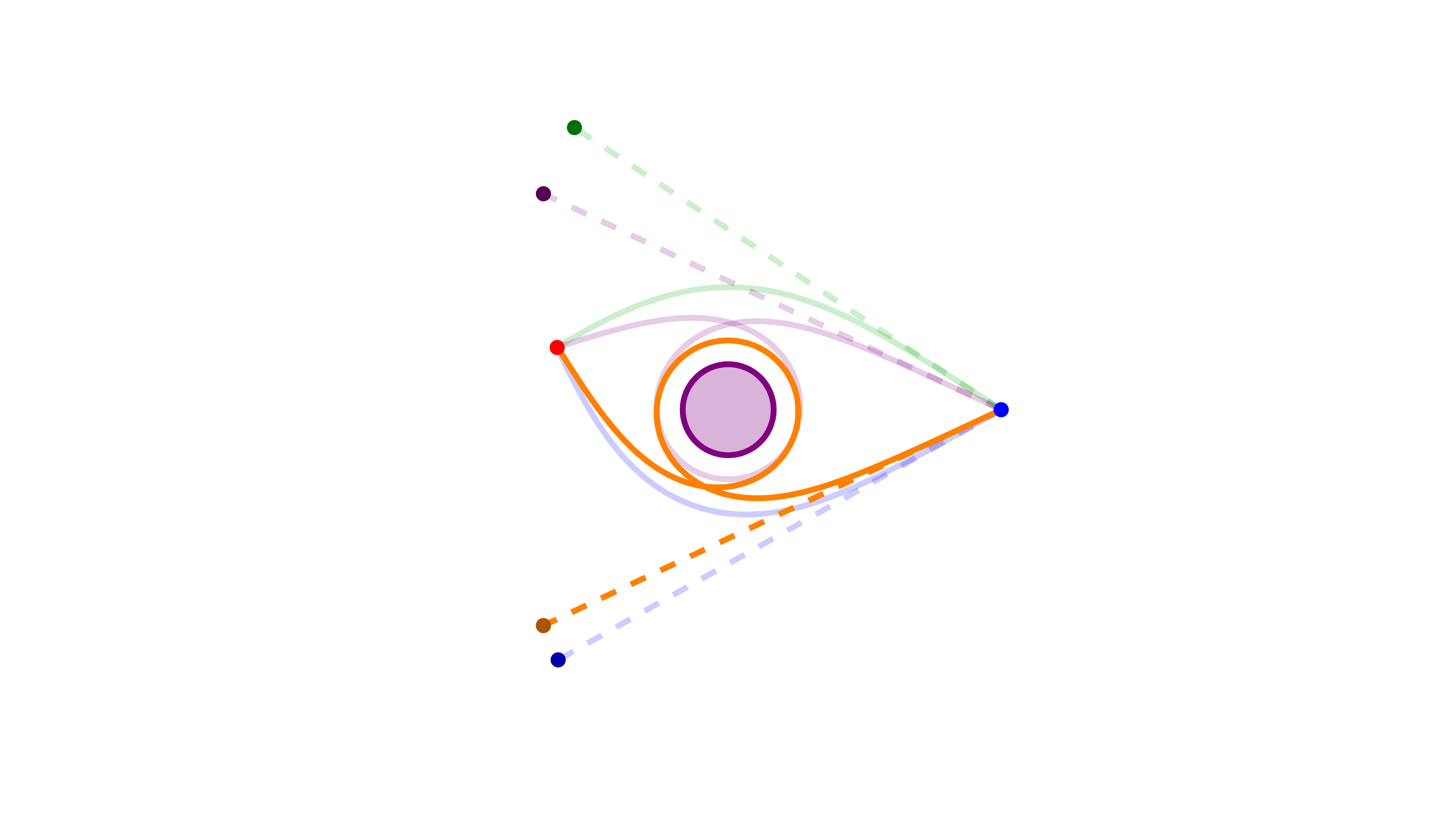
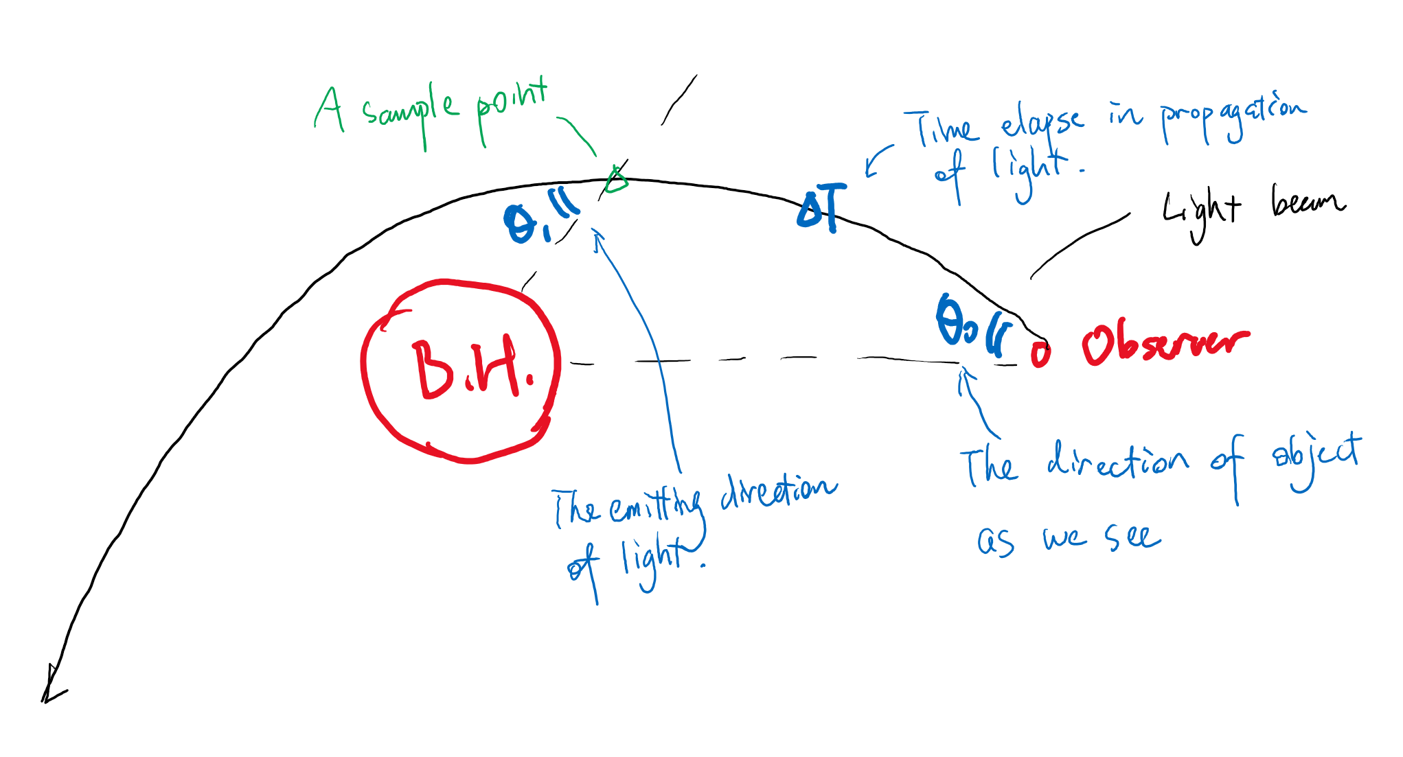
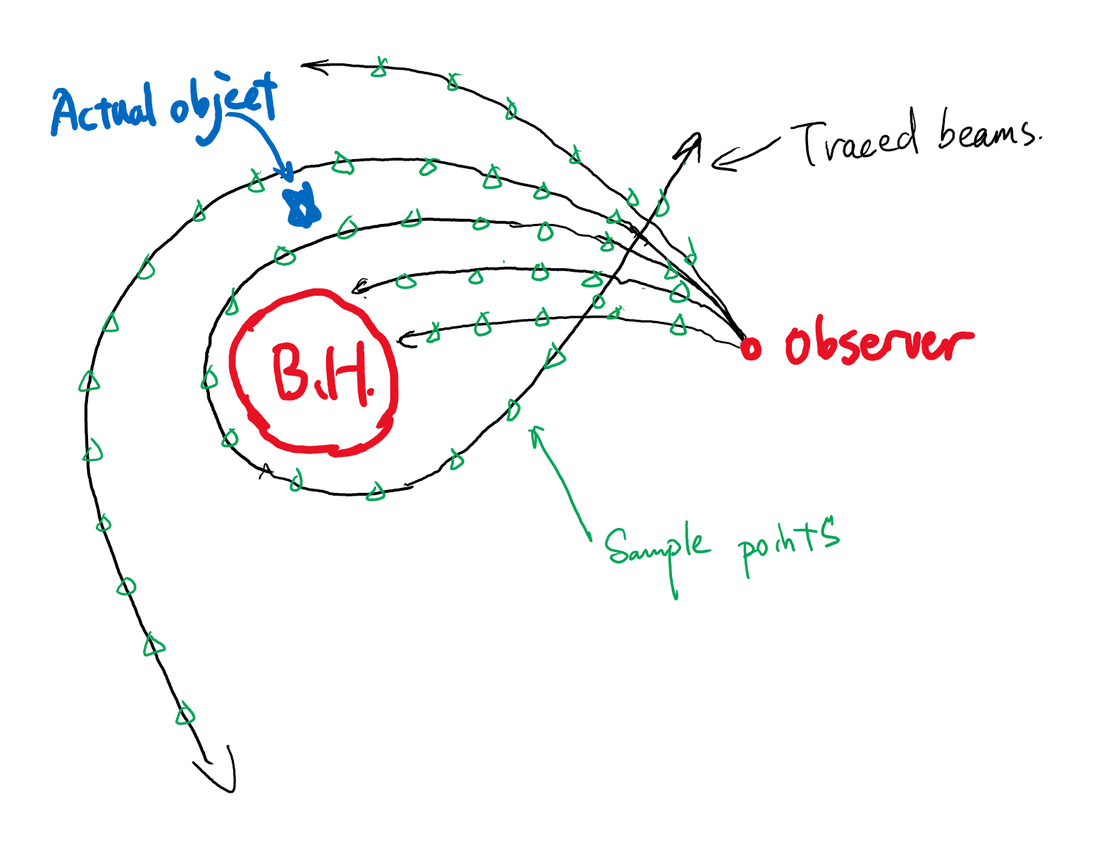
On each ray, we take some sample points and record the corresponding angle $\theta_0$, $\theta_1$, and time $\Delta T$. By interpolating them, we know about how a random object will look like in our eyes.
(*Initial definitions*)
Rs = 1;
R0 = 6 Rs;
Rmax = 6 Rs + 1.*^-6;
(*Tracking the light*)
parfunc =
  ParametricNDSolveValue[{{tt''[\[Tau]],
      rr''[\[Tau]], \[Theta]\[Theta]''[\[Tau]]} == {(
      Derivative[1][rr][\[Tau]] Derivative[1][tt][\[Tau]])/(
      rr[\[Tau]] - rr[\[Tau]]^2), (
       rr[\[Tau]]^2 Derivative[1][
          rr][\[Tau]]^2 - (-1 + rr[\[Tau]])^2 Derivative[1][
          tt][\[Tau]]^2)/(
       2 (-1 + rr[\[Tau]]) rr[\[Tau]]^3) + (-1 +
          rr[\[Tau]]) Derivative[1][\[Theta]\[Theta]][\[Tau]]^2, -((
       2 Derivative[1][rr][\[Tau]] Derivative[
         1][\[Theta]\[Theta]][\[Tau]])/rr[\[Tau]])}, {tt'[0],
      rr'[0], \[Theta]\[Theta]'[
       0]} == {1/(1 - Rs/R0), -Cos[\[Theta]0],
      Sqrt[1/(1 - Rs/R0)]/R0 Sin[\[Theta]0]}, {tt[0],
      rr[0], \[Theta]\[Theta][0]} == {0, R0, 0},
    WhenEvent[
     1.01 Rs >= rr[\[Tau]] ||
      rr[\[Tau]] >= Rmax || \[Theta]\[Theta][\[Tau]] >= 3.1 Pi,
     "StopIntegration"]}, {tt[\[Tau]],
    rr[\[Tau]], \[Theta]\[Theta][\[Tau]]}, {\[Tau], 0,
    1000}, {\[Theta]0}];
(*data used in interpolation*)
datp = Catenate@
   Table[With[{pf = parfunc[\[Theta]]},
     With[{\[Tau]max = pf[[1, 0, 1, 1, 2]], df = D[Rest@pf, \[Tau]],
       f = Rest@pf},
      Block[{\[Tau] =
         Range[RandomReal[{0, \[Tau]max/500}], \[Tau]max, \[Tau]max/
           500]}, Select[
        Thread[(Thread@f ->
           Thread@{\[Theta],
             ArcTan[-df[[1]], df[[2]] f[[1]] Sqrt[1 - Rs/f[[1]]]],
             pf[[1]]})],
        2.4 Rs < #[[1, 1]] < 5.6 Rs && -0.05 Pi < #[[1, 1]] <
           3.08 Pi &]]]], {\[Theta],
     Range[-2.5 Degree, 80 Degree, 1 Degree]~Join~
      Range[20.2 Degree, 28.2 Degree, 0.5 Degree]~Join~
      Range[23.025 Degree, 24.05 Degree, 0.05 Degree]~Join~
      Range[23.2825 Degree, 23.4 Degree, 0.005 Degree]~Join~
      Range[23.28525 Degree, 23.30025 Degree, 0.001 Degree]}];
datp = First /@ GatherBy[datp, Floor[#[[1]]/{0.01 Rs, 1 Degree}] &];

(*Construct InterpolatingFunctions*)
ReceiveAngleFunction =
  Interpolation[Thread[{datp[[;; , 1]], datp[[;; , 2, 1]]}],
   InterpolationOrder -> 1];
EmitAngleFunction =
 Interpolation[Thread[{datp[[;; , 1]], datp[[;; , 2, 2]]}],
  InterpolationOrder -> 1];
DelayFunction =
 Interpolation[Thread[{datp[[;; , 1]], datp[[;; , 2, 3]]}],
  InterpolationOrder -> 1];
(*Angle vs time of observation*)
GenerateAngleFunctions[R1_, \[Theta]1_] := Block[{\[Phi]1},
  With[{interpol =
       Interpolation@
        Table[{DelayFunction[R1, #] +
           Sqrt[2 R1^3] \[Phi]1, \[Phi]1}, {\[Phi]1, 0., 2 Pi,
          10. Degree}]},
     With[{ts = interpol[[1, 1, 1]], tperiod = 2. Pi Sqrt[2 R1^3]},
      Function[t, interpol[t - Floor[t - ts, tperiod]]]]] & /@ ({#,
       2 Pi - #, 2 Pi + #} &@ArcCos[Sin[\[Phi]1] Sin[\[Theta]1]])]
If we only consider this effect, then we will have something like this:
The inner two rings correspond to the light that rotates around the black hole for more than half a round.
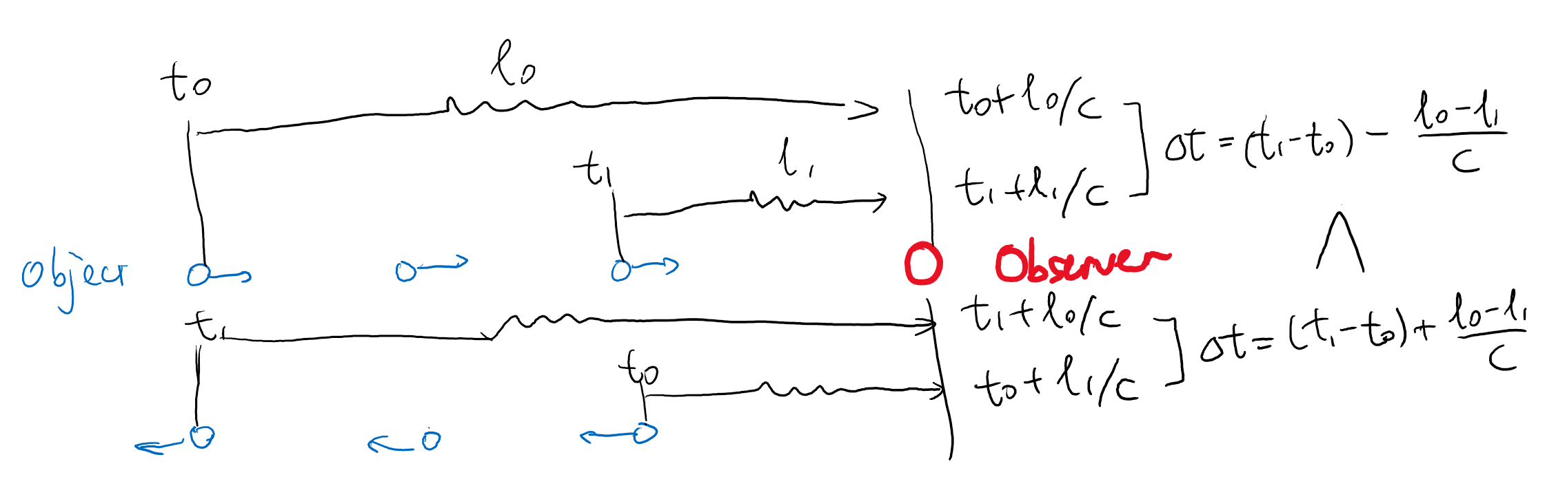
And if we consider the propagation time of light, the right side will be a bit brighter.
This is because on the right, objects are moving away from you. So from your point of view, these particles will stay for a longer time on the right. (The reason is explained in the figure)
"Brighter when Closer"
The next question is about the "brighter when closer" rule. We all know that the further a bulb is, the dimmer it would appear to be. This is because the light from the bulb is approximately evenly distributed across solid angles, but as we move further, the solid angle corresponding to our eyes will be smaller. Mathematically, this is saying $I\propto S_0 \frac{d\Omega}{dS}$ where $S_0$ is the surface area of our eyes, $S$ is area, and $\Omega$ is the solid angle.
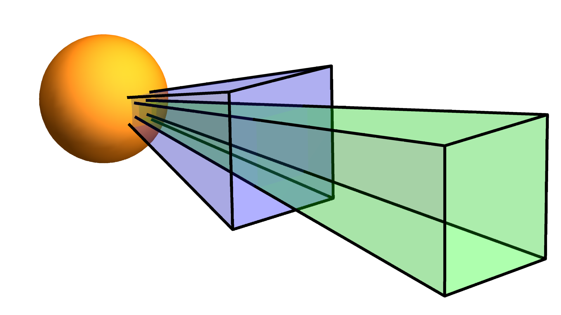
The same rules apply here in curved spacetime, except the light beams are weirder.
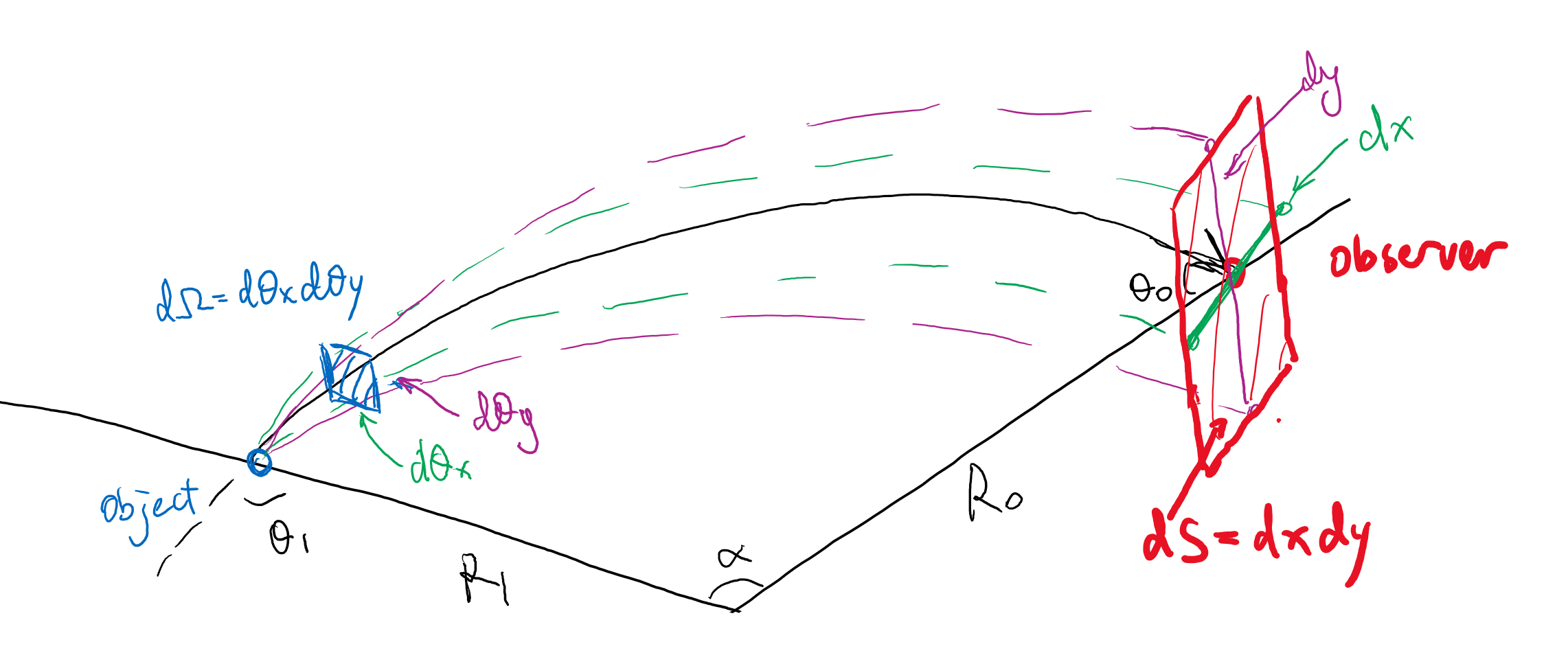
We know that $\frac{d\Omega}{dS}=(\frac{dx}{d\theta_x}\frac{dy}{d\theta_y})^{-1}$. While $\frac{dy}{d\theta_y}=\frac{R_0 \sin \alpha}{\sin \theta_1}$ can be derived using basic solid geometry, $\frac{dx}{d\theta_x}$ must be calculated numerically by tracing the light from the object to the observer. Similarly, we use interpolating function to generalize the result from a set of sample points to the whole space.
(*Reverse ray tracing*)
parfuncrev =
  ParametricNDSolveValue[{{tt''[\[Tau]],
      rr''[\[Tau]], \[Theta]\[Theta]''[\[Tau]]} == {(
      Derivative[1][rr][\[Tau]] Derivative[1][tt][\[Tau]])/(
      rr[\[Tau]] - rr[\[Tau]]^2), (
       rr[\[Tau]]^2 Derivative[1][
          rr][\[Tau]]^2 - (-1 + rr[\[Tau]])^2 Derivative[1][
          tt][\[Tau]]^2)/(
       2 (-1 + rr[\[Tau]]) rr[\[Tau]]^3) + (-1 +
          rr[\[Tau]]) Derivative[1][\[Theta]\[Theta]][\[Tau]]^2, -((
       2 Derivative[1][rr][\[Tau]] Derivative[
         1][\[Theta]\[Theta]][\[Tau]])/rr[\[Tau]])}, {tt'[0],
      rr'[0], \[Theta]\[Theta]'[0]} == {1/(1 - Rs/R1),
      Cos[\[Theta]0], -Sqrt[1/(1 - Rs/R1)]/R1 Sin[\[Theta]0]}, {tt[0],
       rr[0], \[Theta]\[Theta][0]} == {0, R1, \[Theta]1},
    WhenEvent[\[Theta]\[Theta][\[Tau]] == 0,
     "StopIntegration"]}, {tt[\[Tau]],
    rr[\[Tau]], \[Theta]\[Theta][\[Tau]]}, {\[Tau], 0,
    100}, {\[Theta]0, R1, \[Theta]1}];
(*data used in interpolation*)
\[CapitalDelta]\[Phi] = 1.*^-5;
intensity =
  Catenate@Table[{{R, \[Theta]},
     R0^2 With[{\[Theta] = Abs[\[Theta]]},
       Abs[Sin[EmitAngleFunction[
            R, \[Theta]]]/(R0 \
Sin[\[Theta]])]*(\[CapitalDelta]\[Phi]/(Sin[
             ReceiveAngleFunction[R, \[Theta]]]*
            Subtract @@ (With[{f =
                   parfuncrev[
                    EmitAngleFunction[
                    R, \[Theta]] + # \[CapitalDelta]\[Phi],
                    R, \[Theta]][[2, 0]]}, f@f[[1, 1, -1]]] & /@ {-1,
                1})))]}, {R, 2.45 Rs, 5.55 Rs,
     0.02 Rs}, {\[Theta], -3 Degree, 543 Degree, 2 Degree}];

(*Construct InterpolatingFunction*)
IntensityFunction1 = Interpolation[intensity];
The figure will be much more realistic in the aspect of intensity after we added this effect. The inner two rings are much dimmer because light bent dramatically is rare after all.
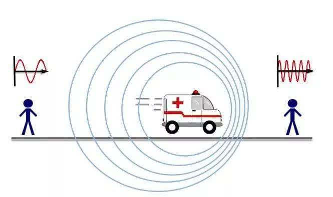
Doppler Effect and Headlight Effect
Now its time for Doppler effect and headlight effect. These two effects are related to the movement of light-emitting objects and observers. Though the names of these effects can be forbidding, these effects are quite common in everyday life. Blueshift refers to the phenomenon that when a car is approaching you, the noise made by the car would be more acute and loud, and redshift means when the car is leaving you, the noise would quieter and be of lower frequency.
The equation for the relativistic Doppler effect is:
$$ f'=f\frac{\sqrt{1-\beta^2}}{1-\beta \cos \theta} $$
where $\beta=\frac{v}{c}$ and $\theta$ is the angle between the velocity direction of the light-emitting object and the light emitted, as observed by an external observer. In this case, we should further add a coefficient of
$$ f''=f'\sqrt{\frac{1 - Rs/R1}{1 - Rs/R0}} $$
due to general relativistic effects.
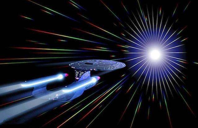
Headlight effect means when you are driving a car on rainy days, no matter how the wind blows, the raindrops will always run towards the windshield. But if you stop your vehicle, you can see how the wind influences the dropping direction of rain.
The equation for angle transformation is:
$$ \cos \theta'= \frac{\cos \theta +\beta}{1+\beta \cos \theta} $$
and such, the intensity difference introduced by this can be written as:
$$ \frac{dP'}{d\Omega}= \frac{dP}{d\Omega}\frac{\sin \theta}{\sin \theta'}\frac{d \theta}{d \theta'}=\frac{dP}{d\Omega}\frac{1 - \beta^2}{(1 -\beta \cos \theta)^2} $$
Except for the difference in timing brought by the curved spacetime, these two effects are purely in the special relativity regime. The only thing involved in coding is tedious coordinate transformation.
(*Calculate moving speed*)
Calc\[Beta][{R1_, \[Theta]_, \[Phi]_}, {vr_, v\[Theta]_, v\[Phi]_}] :=
  Sqrt[vr^2/(1 -
       Rs/R1) + (R1 v\[Theta])^2 + (R1 Sin[\[Theta]] v\[Phi])^2]/
  Sqrt[1 - Rs/R1]
(*Calculate inner product between moving direction and light direction*)
CalcCosAngle[{R1_, \[Theta]_, \[Phi]_}, {vr_, v\[Theta]_, v\[Phi]_}] :=
  With[{v = {vr/Sqrt[1 - Rs/R1], R1 v\[Theta],
     R1 Sin[\[Theta]] v\[Phi]}},
  MapThread[With[{\[Theta]0 = EmitAngleFunction[R1, #1]},
     With[{vnormed = MapThread[Normalize@*List, v]},
      MapThread[
       Dot, {vnormed, Thread@{Cos[\[Theta]0], #2 Sin[\[Theta]0], 0}},
       1]]] &, {{\[Theta], 2 Pi - \[Theta], 2 Pi + \[Theta]}, {-1,
     1, -1}}]]
(*Frequency shift, Doppler effect + GR timing effects*)
FrequencyMult[R1_, \[Beta]_, cos_] :=
 Sqrt[(1 - Rs/R1)/(1 - Rs/R0)]*Sqrt[1 - \[Beta]^2]/(1 - \[Beta] cos)
(*Intensity shift due to headlight effect only*)
IntensityMult2[\[Beta]_,
  cos_] := (Sqrt[1 - \[Beta]^2]/(1 - \[Beta] cos))^2
Then we can put all these effects together and see how things works out!
<< PhysicalColor`

IntensityFunctionScaling::usage = "Scale Intensity.";
Protect@IntensityFunctionScaling;

Options[RenderFunc] = {ColorFunction -> TemperatureColor,
   ColorFunctionScaling -> (# &), IntensityFunctionScaling -> (# &),
   "StaticObserver" -> True};

RenderFunc[R1_, {\[Theta]1_, t1_, \[Gamma]1_}, {T0_, I0_},
  OptionsPattern[]] :=
 Function[t, Through[#[t]]] &@Module[{
    (*Velocity of observer*)
    vobs = N@Sqrt[(1 - Rs/R0) Rs/(2 R0)],
    (*list of \[Phi]1 parameters*)
    \[Phi]1l = Range[0., 2 Pi, 1 Degree],
    (*Polar coordinates \[Theta] and \[Phi]*)
    \[Theta]l0, \[Phi]l0,
    (*velocity of object and its norm*)
    vrl, v\[Theta]l, v\[Phi]l, vnorml
    },
   (*Polar coordinate \[Theta]*)
   \[Theta]l0 = ArcCos[Sin[\[Phi]1l] Sin[\[Theta]1]];

   (*Original \[Phi]*)
   \[Phi]l0 =
    ArcTan[Cos[\[Phi]1l], Sin[\[Phi]1l] Cos[\[Theta]1]] + \[Gamma]1;

   (*velocity of object*)
   vrl = ConstantArray[0, Length@\[Phi]1l];
   v\[Theta]l = -(Cos[\[Phi]1l] Sin[\[Theta]1])/
      Sqrt[1 - Sin[\[Theta]1]^2 Sin[\[Phi]1l]^2]*Sqrt[Rs/(2 R1^3)];
   v\[Phi]l =
    1/(Cos[\[Phi]1l]^2/Cos[\[Theta]1] +
        Cos[\[Theta]1] Sin[\[Phi]1l]^2)*Sqrt[Rs/(2 R1^3)];

   (*velocity norm*)
   vnorml =
    Calc\[Beta][{R1, \[Theta]l0, 0}, {vrl, v\[Theta]l, v\[Phi]l}];

   MapThread[Module[{
       (*Observed \[Phi]1 parameter - t*)
       \[Phi]1t = #3,
       (*actual \[Theta] of object*)
       \[Theta]l = #1,
       (*angle between velocy and ray*)
       cosl = #4,
       (*Observed values - \[Phi]1*)
       (*Geometry*)
       \[Theta]obsl, \[Phi]obsl = \[Phi]l0 + #2,
       (*Frequency and intensity shift*)
       freqobsl, intobsl,
       (*helper function*)
       helpf
       },
      \[Theta]obsl = ReceiveAngleFunction[R1, \[Theta]l];

      (*Frequency*)
      freqobsl = FrequencyMult[R1, vnorml, cosl];

      (*Process with the non-static observer*)
      If[OptionValue["StaticObserver"] =!= True,
       Module[{\[Theta]transl, \[Phi]transl, \[Delta] = ArcSin[vobs]},
        (*Geometrics, static frame*)
        \[Theta]transl = ArcCos[Sin[\[Theta]obsl] Cos[\[Phi]obsl]];
        \[Phi]transl =
         ArcTan[Sin[\[Theta]obsl] Sin[\[Phi]obsl], Cos[\[Theta]obsl]];
        (*Frequency shift due to movement of observer,
        intensity shift is calculated together later*)
        freqobsl *= (1 + vobs Cos[\[Theta]transl])/Sqrt[1 - vobs^2];
        (*Angle shift due to movement of observer*)
        \[Theta]transl =
         ArcCos[(vobs + Cos[\[Theta]transl])/(1 +
             vobs Cos[\[Theta]transl])];
        (*Transform back*)
        (*Here we change the center of viewing angle so that the \
black hole's center is at {0,0}*)
        \[Theta]obsl =
         ArcCos[Sin[\[Delta]] Cos[\[Theta]transl] +
           Cos[\[Delta]] Sin[\[Theta]transl] Sin[\[Phi]transl]];
        \[Phi]obsl =
         ArcTan[Cos[\[Delta]] Cos[\[Theta]transl] -
           Sin[\[Delta]] Sin[\[Theta]transl] Sin[\[Phi]transl],
          Sin[\[Theta]transl] Cos[\[Phi]transl]]
        ]
       ];

      \[Phi]obsl =
       Catenate[
        MapIndexed[#1 + 2 Pi #2[[1]] &, Split[\[Phi]obsl, Less]]];

      (*Intensity*)
      intobsl =
       freqobsl^2*IntensityFunction1[R1, \[Theta]l]*
        IntensityMult2[vnorml, cosl]*
        TemperatureIntensity[freqobsl T0]/TemperatureIntensity[T0]/
         freqobsl^4;

      (*Helper function to construct interpolating functions*)
      helpf[l_] := Interpolation[Thread[{\[Phi]1l, l}]];

      With[{
        cf = OptionValue[ColorFunction],
        (*Interpolating functions*)
        t11 = t1,
        \[Phi]1f = #3,
        \[Theta]func = helpf[\[Theta]obsl],
        \[Phi]func = helpf[\[Phi]obsl],
        freqfunc =
         helpf[OptionValue[ColorFunctionScaling][T0 freqobsl]],
        intfunc =
         helpf[OptionValue[IntensityFunctionScaling][I0 intobsl]]
        },

       (*Final function*)
       Function[t,
        With[{\[Phi]11 = \[Phi]1f[t + t11]},
         {Append[cf[freqfunc[\[Phi]11]], intfunc[\[Phi]11]],

          With[{\[Theta] = \[Theta]func[\[Phi]11], \[Phi] = \
\[Phi]func[\[Phi]11]},
           (*Point[{Sin[\[Theta]]Cos[\[Phi]],Sin[\[Theta]]Sin[\[Phi]],
           Cos[\[Theta]]}]*)
           Point[Tan[\[Theta]] {Cos[\[Phi]], Sin[\[Phi]]}]]}
         ]]
       ]
      ] &, {{\[Theta]l0, 2 Pi - \[Theta]l0, 2 Pi + \[Theta]l0}, {0,
      Pi, 0}, GenerateAngleFunctions[R1, \[Theta]1],
     CalcCosAngle[{R1, \[Theta]l0, 0}, {vrl, v\[Theta]l, v\[Phi]l}]}]]
(*My version of rasterize, which increase color precision in dimmer areas*)
HDRRasterize[gr_Graphics, convertfunc_,
  opts : OptionsPattern[Rasterize]] :=
 Module[{rasterl =
    Join[ColorSeparate[ColorConvert[Rasterize[gr, opts], "HSB"]],
     ColorSeparate[
      ColorConvert[
       Rasterize[
        gr /. RGBColor[r_, g_, b_, op_] :> RGBColor[r, g, b, 16 op],
        opts], "HSB"]]], mask, invmask},
  mask = Binarize[rasterl[[3]], 1/16];
  invmask = 1 - mask;
  ColorCombine[{
    mask*rasterl[[1]] + invmask*rasterl[[4]],
    mask*rasterl[[2]] + invmask*rasterl[[5]],
    mask*convertfunc[rasterl[[3]]] +
     invmask*convertfunc[rasterl[[6]]/16.]}, "HSB"]
  ]
(*Preliminary computation*)
npts = 5000;
rflist = MapThread[
   Function[{R1, \[Theta]1, t1, \[Gamma]1, T0, I0},
    RenderFunc[R1, {\[Theta]1, t1, \[Gamma]1}, {T0, I0},
     "StaticObserver" -> False(*,
     IntensityFunctionScaling\[Rule](.7(#/.5)^0.5&)*)]],
   {RandomReal[{3, 4.5}, npts],
    RandomReal[-{83, 86} Degree, npts],
    RandomReal[{0, 10000}, npts],
    RandomReal[15 Degree + {-2, 2} Degree, npts],
    RandomReal[{4000, 10000}, npts],
    RandomReal[{.03, .1}, npts]
    }
   ];
(*rendering!!!*)
g = Graphics[{(*AbsolutePointSize@.1,White,Point[{Sin[20Degree]Cos[#],
    Sin[20Degree]Sin[#],Cos[20Degree]}&/@Range[0.,360.Degree,
    60.Degree]],*)AbsoluteThickness@2,
    Map[Line[#[[;; , 2, 1]],
       VertexColors ->
        MapThread[
         Function[{col, len, mult},
          MapAt[mult^2*#*0.006/len &, col, 4]], {#[[;; , 1]],
          Prepend[#, #[[1]]] &@
           BlockMap[Norm[#[[2]] - #[[1]]] &, #[[;; , 2, 1]], 2, 1],
          Subdivide[Length[#] - 1]}]] &,
     Reverse@Transpose[
       Through[rflist[#]] & /@ (Range[0, 3, .1]), {3, 2, 1}], {2}]},
   Background -> Black, ImageSize -> {500, Automatic},
   PlotRange -> {{-1.28, 1.28}, {-0.72, 0.72}}];

HDRRasterize[g, #^(1/2.2) &, ImageSize -> {1920, 1080}]
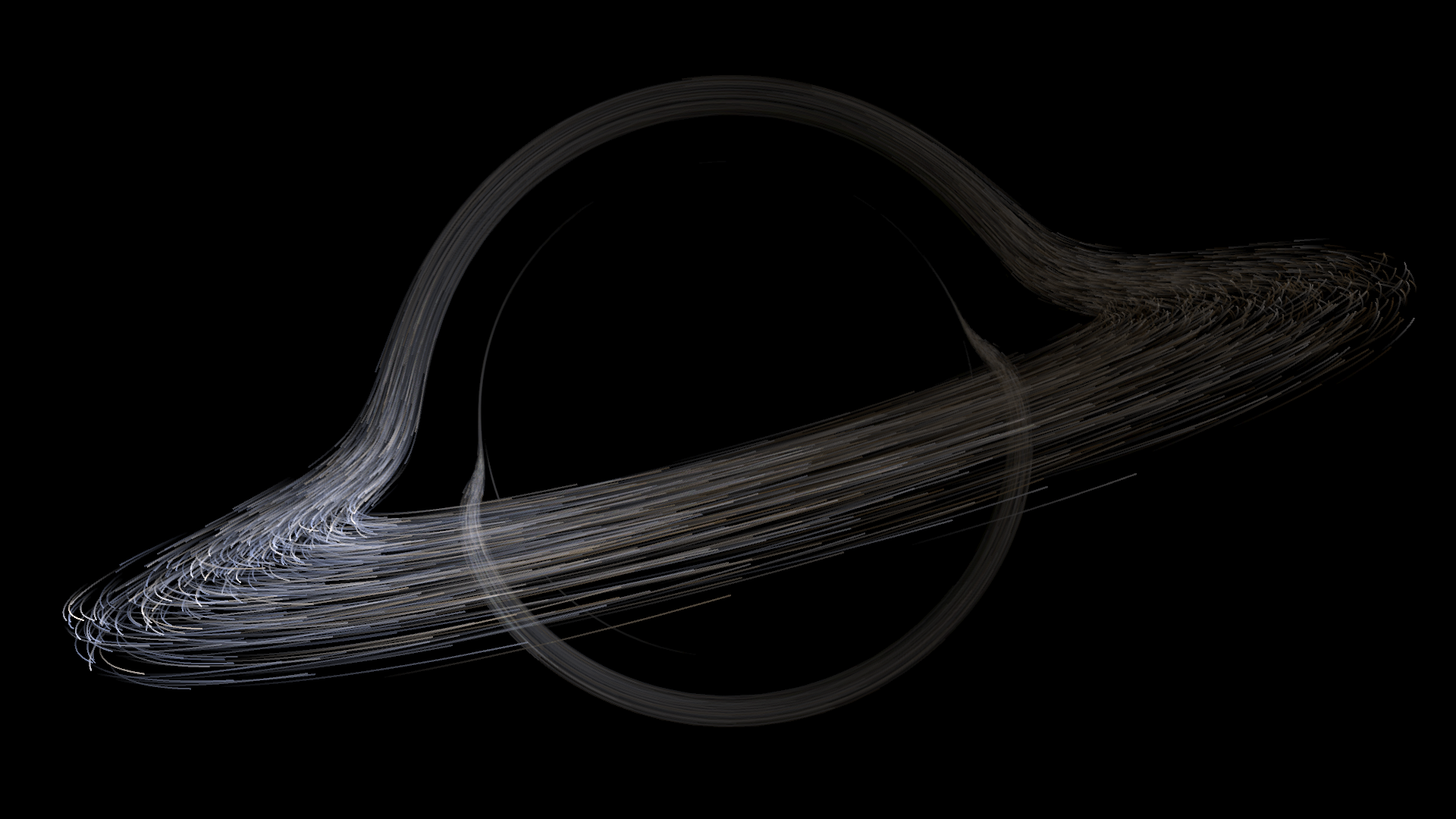
Well, because objects at left are moving towards you, they will appear much brighter and blue-ish, while objects at right are much dimmer and red-ish.
We can also consider the movement of the observer, which will make the image something like this:
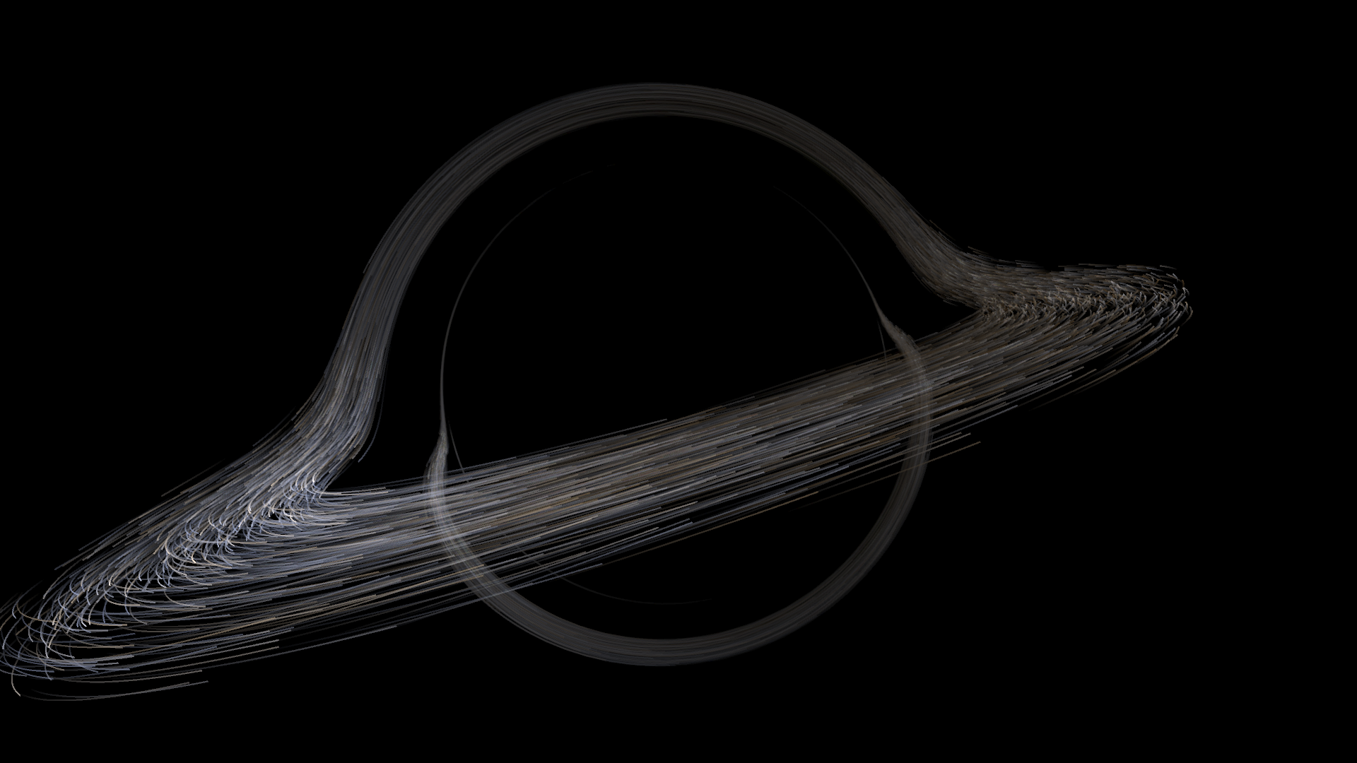
Hooray!
The notebook can be found in the attachment or at my github repo.
 Attachments:


