
In a previous Wolfram Demonstration Pendulum with Varying Length or How to Improve Your Next Swing Ride, I modelled a swing and rider system as a pendulum with varying length. Inspired by the article "Pumping a Playground Swing" by Post et al. I looked at an alternative strategy to "optimize my swing ride". The swing-rider system can be modeled as a double pendulum. The regular, unforced double pendulum maintains a constant level of energy. Kinetic-and potential energy are merely converted into one another and their sum remains constant. In the case of a swing however, we have a forced double pendulum as the rider wants to go higher and "pump" his way up. This can only be achieved by increasing the total energy in the (swing and rider) system. "Energy insertion" can be done by someone pushing the rider or by a properly synchronized change in the position of the center of mass (CM) of the rider. In the mentioned demonstration, the CM change was limited to an up and down crouching of the rider. Here, I will analyse a more general, circular or elliptic position change of the rider's CM.
Geometry
Let us first look at the geometry of the swing-rider system: The swinging kid at P can introduce energy into the double pendulum by forcibly moving his center of gravity in an elliptic movement around a point Z on the rigid swing rods OS. [Theta] is the angle of the swing movement and [Phi] is the angle of the crouching movement (rotation). We need a "crouching function" linking the angles [Phi] and [Theta]: [Phi] = [Omega] [Theta]+[Phi]0. [Omega] is the crouching frequency and [Phi]0 is the crouching's initial angular offset.
Animate[
 With[{L = 10, r = 2., \[Omega] = 3., \[Phi]0 = 0, a = .62, b = 2},
  Module[{pivot, \[Phi], trace, seatCenter, hipPivot, hip},
   pivot = {0, 0}; \[Phi] = \[Omega] \[Theta] + \[Phi]0;
   seatCenter = {L Sin[\[Theta]], -L Cos[\[Theta]]};
   hipPivot = (L - r) {Sin[\[Theta]], -Cos[\[Theta]]};
   hip = {(L - r - a Cos[\[Phi]]) Sin[\[Theta]] +
      b Cos[\[Theta]] Sin[\[Phi]],
     Cos[\[Theta]] (-L + r + a Cos[\[Phi]]) +
      b Sin[\[Theta]] Sin[\[Phi]]};
   trace = Rotate[Circle[hipPivot, {b, a}], \[Theta]];
   Graphics[{Line[{pivot, seatCenter}], Blue, Line[{hipPivot, hip}],
     PointSize[.015],
     Point[{pivot, hip, hipPivot, seatCenter}], {Red, trace}, {Dashed,
       Line[{hip, pivot}]},
     {Black, Text[Style["O", 12], pivot, {-1, -1}],
      Text[Style["Z", 12], hipPivot, {1, 1}],
      Text[Style["P", 12], hip, {-1, -1}],
      Text[Style["S", 12], seatCenter, {-1, 1}]}}]]], {\[Theta], 0,
  2 Pi}]
Dynamic Model
We add the driver's mass mk at P and consider the crouching as a periodic driving force. We use Newton's laws to derive the equation of motion:
(*hip (CM) coordinate*)
xh[t_] :=
  b Cos[\[Theta][t]] Sin[\[Phi]0 + t \[Omega]] + (L - r -
      a Cos[\[Phi]0 + t \[Omega]]) Sin[\[Theta][t]];
yh[t_] := (-L + r + a Cos[\[Phi]0 + t \[Omega]]) Cos[\[Theta][t]] +
   b Sin[\[Phi]0 + t \[Omega]] Sin[\[Theta][t]];
(*effective swing length*)l = Sqrt[xh[t]^2 + yh[t]^2];
(*equilibrium of forces*)
deqns = {mk xh''[t] == s[t] xh[t]/l,
   mk yh''[t] == s[t] yh[t]/l - mk g};
deqn = Eliminate[deqns, s[t]] // FullSimplify
This is an animation showing a solution of the differential equation. The evolution of the energy levels shows how the forced position changes in the rider's CM is increasing the total energy in the system. Trying to reach a large energy increase in a short time is the goal of every swing rider. Here, a maximum energy level with a high swing is reached after a mere 1.5 full swings.
Animate[Module[{a = 1.75,
   b = 1.5, \[Omega] = 1.9, \[Phi]0 =
    0, \[Theta]0 = \[Pi]/4, \[Theta]00 = 0, V, T, mk = 50, g = 9.81,
   L = 10, l, xh, yh, \[Theta]sol, seat, hip, hipPivot, trace,
   tMax = 16, r = .75},
  pivot = {0, 0};
  (*crouch function*)\[Phi][t_] := \[Omega] t + \[Phi]0;
  xh[t_] :=
   b Cos[\[Theta][t]] Sin[\[Phi]0 + t \[Omega]] + (L - r -
       a Cos[\[Phi]0 + t \[Omega]]) Sin[\[Theta][t]];
  yh[t_] := (-L + r + a Cos[\[Phi]0 + t \[Omega]]) Cos[\[Theta][t]] +
    b Sin[\[Phi]0 + t \[Omega]] Sin[\[Theta][t]];
  sol = First@
    NDSolve[{deqn, \[Theta][0] == \[Theta]0, \[Theta]'[
        0] == \[Theta]00}, \[Theta], {t, 0, tMax}];
  hip = {xh[t], yh[t]} /. sol /. t -> time;
  seat = L {Sin[\[Theta][time]], -Cos[\[Theta][time]]} /. sol;
  hipPivot = (L - r) {Sin[\[Theta][time]], -Cos[\[Theta][time]]} /.
    sol;
  trace = Rotate[Circle[hipPivot, {b, a}], \[Theta][time]] /. sol;
  (*kinetic energy*)
  T[t_] := Evaluate[.5 mk (xh'[t]^2 + yh'[t]^2)] /.
    sol;(*potential energy*)V[t_] := mk g yh[t] /. sol;
  Column[{
    Plot[Evaluate[{V[t], T[t] + V[t]}], {t, 0, tMax},
     Filling -> {2 -> {1}, 1 -> Bottom}, PlotLabel -> "Energy",
     PlotLegends -> Placed[{"Potential", "Total"}, Bottom],
     AxesLabel -> {"t", ""},
     Epilog -> {AbsoluteThickness[.75],
       Line[{{time, -10000}, {time, 10000}}]}],
    Graphics[{(*support*){FaceForm[Yellow], EdgeForm[Black],
       Triangle[{pivot, 10 {-.035, .045}, 10 {.035, .045}}], Red,
       Disk[pivot, .01]},
      (*floor*), {Brown, AbsoluteThickness[4],
       Line[{{-10, -L - a}, {10, -L - a}}]},
      Point[{pivot, seat, hipPivot}],
      Line[{pivot, hip}], {Directive[Blue, AbsoluteThickness[.5]],
       trace}, {DotDashed, Line[{pivot, seat}]}, {Blue,
       Line[{hipPivot, hip}]}, {Red, AbsolutePointSize[7], Point@hip,
       White, Disk[hip, .025]},
      ParametricPlot[
        Evaluate[{xh[t], yh[t]} /. sol], {t, 0, time + .001},
        PlotStyle -> Directive[Red, AbsoluteThickness[.75]]][[1]]},
     PlotRange -> 12, Axes -> True]}]], {time, 0, 15.5, .25}]
Adding a rider
I designed a simplified rider figure with the hip position at the center of gravity and fixed points where the foot is on the seat and the grip of the hand is on the front rod. This figure can then simply be fitted into the previous code to make a working and more realistic model.
kidNSwing[hip : {hx_, hy_}] :=

 With[{pivot = {0, 0}, L = 10, seat = .75, head = .45, grip = 2.5,
   leg = 1.55, thigh = 1.4, trunk = 1.5, arm1 = 1.25, arm2 = 1.2},
  Module[{(*joints*)ptF, ptB, ptT, ptS, ptK, ptP, ptN, ptE, ptH,
    ptD},
   ptT = {-.2, -L}; ptS = {0, -L + .085}; ptF = {-seat, -L};
   ptB = {seat, -L}; ptK = findTop[ptS, hip, leg, thigh];
   ptH = AngleVector[{(L - grip), -1.6458}];
   ptN = First@
     Nearest[{x, y} /.
       Solve[{x, y} \[Element] Line[{ptS, pivot}] &&
         EuclideanDistance[{x, y}, hip] == trunk + .1, {x, y}], pivot];
   ptE = findTop[ptN, ptH, arm2, arm2];
   ptD = First@
     Nearest[{x, y} /.
       Solve[{x, y} \[Element] Line[{ptN, pivot}] &&
         EuclideanDistance[{x, y}, hip] == trunk + head + .175, {x,
         y}], pivot];
   {(*seat*){AbsoluteThickness[6], Gray, Line[{ptF, ptB}]},
    (*rods*){AbsoluteThickness[.9],
     Line[{ptF, {0, 0}, ptB}]}, {PointSize[.01], Point[hip]},
    (*trunk & limbs*) {FaceForm[Lighter[Red, .8]],
     EdgeForm[AbsoluteThickness[1]],
     StadiumShape[#, .125] & /@
      Partition[{ptT, ptS, ptK, hip, ptN, ptE, ptH}, 2, 1] },
    (*joints*){Disk[#, .12] & /@ {ptT, ptS, ptK,(*hip,*)ptN, ptE,
       ptH}, White,
     Disk[#, .065] & /@ {hip, ptT, ptS, ptK,(*hip,*)ptN, ptE, ptH}},
    (*head*){Darker[Gray, .35],
     Disk[ptD, head, {176 \[Degree], -154 \[Degree]}],(*eye*)White,
     Disk[ptD, .075]}}]]
Full model to Optimize your Swing ride
The equation of motion is then introduced in a Manipulate. This lets the user experiment with a simple model of the swing and rider system to explore the conditions for an optimized swing ride . The parameters of the hip (CM) displacement and the initial conditions (angular position and speed) can be adjusted. The energy level graph on top lets the user see where the maximum energy level occurs and try do move this as much as possible to the start of the ride.
Manipulate[With[{mk = 50, g = 9.81, pivot = {0, 0}, L = 10},
Module[{deqn, crouch, xh, yh, sol, \[Phi], V, T, hipPivot, hip,
trace}, time = Min[tMax, time];
\[Phi][t_] := \[Omega] t + \[Phi]0;
crouch[t_] := {b Sin[\[Phi][t]], -L + r + a Cos[\[Phi][t]]};
xh[t_] :=
b Cos[\[Theta][t]] Sin[\[Phi]0 + t \[Omega]] + (L - r -
a Cos[\[Phi]0 + t \[Omega]]) Sin[\[Theta][t]];
yh[t_] := (-L + r + a Cos[\[Phi]0 + t \[Omega]]) Cos[\[Theta][t]] +
b Sin[\[Phi]0 + t \[Omega]] Sin[\[Theta][t]];
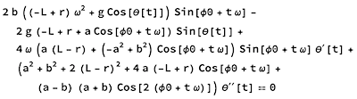
deqn =
2 b ((-L + r) \[Omega]^2 + g Cos[\[Theta][t]]) Sin[\[Phi]0 +
t \[Omega]] +
4 \[Omega] (a (L - r) + (-a^2 + b^2) Cos[\[Phi]0 +
t \[Omega]]) Sin[\[Phi]0 + t \[Omega]] Derivative[
1][\[Theta]][
t] + (a^2 + b^2 + 2 (L - r)^2 +
4 a (-L + r) Cos[\[Phi]0 + t \[Omega]] + (a - b) (a + b) Cos[
2 (\[Phi]0 + t \[Omega])]) (\[Theta]^\[Prime]\[Prime])[
t] == 2 g (-L + r + a Cos[\[Phi]0 + t \[Omega]]) Sin[\[Theta][
t]];
sol = First@
NDSolve[{deqn, \[Theta][0] == \[Theta]0, \[Theta]'[
0] == \[Theta]00}, \[Theta], {t, 0, tMax}];
hip[t_] := {xh[t], yh[t]} /. sol;
hipPivot = (L - r) {Sin[\[Theta][time]], -Cos[\[Theta][time]]} /.
sol;
trace[t_] := Rotate[Circle[hipPivot, {b, a}], \[Theta][t]];
T[t_] := Evaluate[.5 mk (xh'[t]^2 + yh'[t]^2)] /. sol;
V[t_] := mk g yh[t] /. sol;
Column[{
Plot[Evaluate[{V[t], T[t] + V[t]}], {t, 0, tMax},
Filling -> {2 -> {1}, 1 -> Bottom}, PlotLabel -> "Energy",
PlotLegends -> Placed[{"Potential", "Total"}, Bottom],
AxesLabel -> {"t", ""}, AxesStyle -> 7,
Epilog -> {AbsoluteThickness[.75],
Line[{{time, -1*^6}, {time, 1*^6}}]}, ImageSize -> 400,
AspectRatio -> .3],
Graphics[{
{FaceForm[Yellow], EdgeForm[Black],
Triangle[{pivot, {-.35, .45}, {.35, .45}}], Red,
Disk[pivot, .15]},
(*floor*), {Brown, AbsoluteThickness[4],
Line[{{-20, -L - 1}, {20, -L - 1}}]},
ParametricPlot[
hip[t] /. sol, {t, 0, If[sdt, tMax, time + .01]},
PerformanceGoal -> "Quality",
PlotStyle -> Directive[AbsoluteThickness[.45], Red],
PlotPoints -> 10][[1]],
Rotate[kidNSwing[crouch[time]], \[Theta][time], pivot] /. sol,
If[
sht, {Directive[Dashed, Blue, AbsoluteThickness[1.5]],
trace[time] /. sol}, Nothing]},
Background -> Lighter[Gray, 0.8],
Axes -> True, Frame -> True, FrameTicks -> None,
PlotRange -> 1.1 {{-L, L}, {-L - .1, L}},
ImageSize -> 400]}]]],
Style["animation", Bold, 10],
{{time, 0.}, 0., tMax, .001, ImageSize -> Tiny,
Appearance -> "Labeled"}, Delimiter,
Style["swinging", Bold, 10],
"initial angular position kid", {{\[Theta]0, 1.31}, -1.57,
1.57, .001, ImageSize -> Tiny, Appearance -> "Labeled"},
"initial angular speed",
{{\[Theta]00, 0}, -6, 6, .0001, ImageSize -> Tiny,
Appearance -> "Labeled"}, Delimiter,
Style["crouching", Bold, 10],
"major axis a (in line with swing rods)", {{a, .75}, 0., 2, .001,
ImageSize -> Tiny, Appearance -> "Labeled"},
"minor axis b (perpendicular to swing rods)", {{b, .274}, 0.,
2, .001, ImageSize -> Tiny, Appearance -> "Labeled"},
"frequency",
{{\[Omega], 1.904}, -5, 5, .001, ImageSize -> Tiny,
Appearance -> "Labeled"},
"angular offset",
{{\[Phi]0, 0}, -1.57, 1.57, .0001, ImageSize -> Tiny,
Appearance -> "Labeled"}, Delimiter,
"hip vertical offset",
{{r, 1.6722}, 0, 2.5, .0001, ImageSize -> Tiny,
Appearance -> "Labeled"}, Delimiter,
Row[{"show full dynamic trace",
Control[{{sdt, False, ""}, {True, False}}]}],
Row[{"show static trace",
Control[{{sht, False, ""}, {True, False}}]}],
{{tMax, 30, "total time"}, None}, TrackedSymbols :> True,
ControlPlacement -> Left]
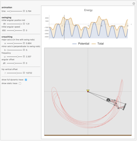
After some experimenting, one can easily derive some conclusions:
the most important effect is to synchronize the crouching ([Phi]) with the swinging ([Theta]). Best results are achieved if the crouching frequency ([Omega]) is double the swing frequency.
up and down crouching (a is the crouching path's semimajor axis in line with swing rods) has more effect than forward- backward leaning (b is the crouching path's semi-minor axis perpendicular to swing rods)
Some Favorite Rides
A start from absolute standstill and zero position. Only the hip movement is in action here and is enough to add energy to the system.
"zero start-1" :> {a = 0.75, b = 0.75,
  r = 1.6722, \[Theta]00 = 0, \[Theta]0 = 0, \[Phi]0 =
   0.253, \[Omega] = 1}
This example also has zero initial speed and position but the crouching is synchronized in a nearly optimal way ([Omega]= approximately 2), resulting in a spectacular swing over the top (we have rigid rods, no ropes or chains!).
"zero start-2" :> {a = 1.2, b = 0,
  r = 1.6722, \[Theta]00 = 0, \[Theta]0 = 0.785, \[Phi]0 =
   0.4664, \[Omega] = 1.994}
Other relations of crouching to swinging can result in some nice periodic rides.
"oval track" :> {a = 0.75, b = 0,
  r = 0.8, \[Theta]00 = 0.0714, \[Theta]0 =
   1.265, \[Phi]0 = -0.2527, \[Omega] = 3.74}
Experiment freely with the previous Manipulate and get as much fun as I did with this simple model of something we are all familiar with.


