Message Boards Message Boards

0
|
8332 Views
|
10 Replies
|
7 Total Likes
View groups...
Share
Share this post:

Error with NonlinearModelFit[ ]?

Posted 3 years ago

Hello, I am a beginner user of Mathematica. I am using Mathematica to plot my ascii.csv file I have obtained through making measurement from a laser beam profiler. I am currently working on my capstone.

I am trying to figure out how to fit my .csv data to a two-dimensional Gaussian fit function. Currently my NonlinearModelFit is not working. Mathematica is giving me a list of errors. I have tried to search the internet, but I may not be searching the right topic since I can't seem to figure out the problem.

One of the errors I am getting is "NonlinearModelFit::fitc: Number of coordinates (1928) is not equal to the number of variables (1)." or "NonlinearModelFit::fitc: Number of coordinates (1928) is not equal to the number of variables (2)."

The code I currently have is this:

data = Import[
   "/Users/Isac/Desktop/CAPSTONE/Isac - NEW Capstone \
Measurements/Change in H/11mmH4mmV/40MHz_0001.ascii.csv", "Data"];

nlm = NonlinearModelFit[data, 
  A Exp[-(((x - x0)^2)/(2 \[Sigma]^2) + ((y - 
            y0)^2)/(2 \[Sigma]^2))], {{\[Sigma], 1928}, {x0, 50}, {y0, 
    50}, {A, 1}}, {x,y}]

Show[ListPlot[data, PlotStyle -> Red, PlotRange -> All], 
 Plot[nlm[x,y], {x, 0, 1928}, {y, 0 ,3500}, PlotRange -> All]]

I can't seem to figure out what is wrong. Any help is appreciated!

P.S. Threw in the data.csv, hopefully this helps!

Very Respectfully, Mr. Isac

**edit: The question has been answered. Thank you all who had helped me and guided me to better understanding in how to use Mathematica with the data that I had. My capstone professor is a busy person, and doesn't have much time to help me. Not sure how I would have figure this out myself without the help from everyone here. Thank you all again.

Attachments:
POSTED BY: Isac Perez
10 Replies
Posted 3 years ago

It appears that you want to fit two very separated surfaces with each surface being proportional in height to a bivariate normal distribution. (You're not fitting a probability distribution but rather just using some functions that happen to be proportional to probability distributions.)

First import the data and follow @Updating Name 's advice by restructuring the data:

data = Import["40MHz_0001.ascii.csv", "Data"];
data = Flatten[Table[{i, j, data[[i, j]]}, {i, 1448}, {j, 1929}], 1];

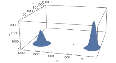
Then (after I snooped a bit at your data) plot the data:

d = Select[data, #[[3]] > 100 &];
ListPointPlot3D[d, PlotRange -> {{250, 1200}, {250, 1200}, {0, 3500}}, AxesLabel -> {"x", "y", "z"}]

Two peaks

Now isolate each peak and use NonlinearModelFit:

data1 = Select[data, 300 < #[[1]] < 650 && 200 < #[[2]] < 500 &];
nlm1 = NonlinearModelFit[data1, {a01 + 
  a1 10^7 PDF[BinormalDistribution[{\[Mu]x1, \[Mu]y1}, {\[Sigma]x1, \[Sigma]y1}, \[Rho]1], {x, y}], a1 > 0},
   {{a01, 35}, {a1, 2}, {\[Mu]x1, 500}, {\[Mu]y1, 350}, {\[Sigma]x1, 35}, {\[Sigma]y1, 35}, {\[Rho]1, 0}}, {x, y}];
nlm1["BestFitParameters"]
(* {a01 -> 61.5589, a1 -> 1.99095, \[Mu]x1 -> 500.052, \[Mu]y1 -> 331.408, \[Sigma]x1 -> 
  34.539, 
  \[Sigma]y1 -> 30.2634, \[Rho]1 -> -0.107371} *)

data2 = Select[data, 350 < #[[1]] < 600 && 800 < #[[2]] < 1200 &];
ListPlot[Select[data2, #[[3]] > 100 &][[All, {1, 2}]]]
nlm2 = NonlinearModelFit[data2, {a02 + 
     a2 10^7 PDF[BinormalDistribution[{\[Mu]x2, \[Mu]y2}, {\[Sigma]x2, \[Sigma]y2}, \[Rho]2], {x, y}], a2 > 0},
   {{a02, 35}, {a2, 1.5}, {\[Mu]x2, 500}, {\[Mu]y2, 1000}, {\[Sigma]x2, 40}, {\[Sigma]y2, 40}, {\[Rho]2, 0}}, {x, y}];
nlm2["BestFitParameters"]
(* {a02 -> 62.7361, a2 -> 1.3379, \[Mu]x2 -> 488.807, \[Mu]y2 -> 1015.64, \[Sigma]x2 -> 
  37.3867, 
  \[Sigma]y2 -> 38.2114, \[Rho]2 -> -0.0203793} *)
POSTED BY: Jim Baldwin
Posted 3 years ago

Thank you so much! This will help me a lot! I have spent days trying to figure this out, reading manuals and articles, but it's hard to know where to start and what to exactly search for when being a beginner with not much experience. This will give me a lot of guidance, since I still have 104 measurement similar (but different) to this one to get done. Thank you again!

POSTED BY: Isac Perez
Posted 3 years ago

One can also find all parameters in a single NonlinearModelFit. If that is desirable, please let me know.

The "secret" to getting NonlinearModelFit to work fine most of the time is to give good starting values. (This is not a Mathematica issue. All iterative methods in all statistics packages have this issue.) So looking at where the approximate peaks are and how spread out they are (the "standard deviation" parameters $\sigma_{x_i}$ and $\sigma_{y_i}$) is critical.

POSTED BY: Jim Baldwin

I wrote some code that allows to estimate the initial values for the fit from the data. Also your function does not allow for certain values so these need to be constrained. And made the function it fits both peaks. Hope it helps.

(*import data and remove string values*)
data = N@DeleteCases[
    Import["C:\\Users\\mfroelin.LA018015\\Desktop\\40MHz_0001.ascii.\
csv", "Data"], "", 2];
(*Put data in list form*)
dataf = Flatten[MapIndexed[Flatten[{#2, #1}] &, data, {2}], 1];
(*plot subset of data*)
datPlot = 
  ListPlot3D[dataf[[;; ;; 1000]], PlotRange -> Full, 
   PlotStyle -> Blue];

(*define the function*)
fun = a0 + 
   a1 PDF[BinormalDistribution[{\[Mu]x1, \[Mu]y1}, {\[Sigma]x1, \
\[Sigma]y1}, \[Rho]1], {x, y}] +
   a2 PDF[
     BinormalDistribution[{\[Mu]x2, \[Mu]y2}, {\[Sigma]x2, \
\[Sigma]y2}, \[Rho]2], {x, y}];

(*find the initial condition*)
{dx, dy} = Dimensions[data];
im = Closing[
   Image[Reverse@
     UnitStep[GaussianFilter[data, 10] - 5 Mean[Flatten[data]]]], 3];
comps = ComponentMeasurements[
   im, {"Centroid", "EquivalentDiskRadius"}];
(*peak location*)
{\[Mu]y1i, \[Mu]x1i} = First[1 /. comps];
{\[Mu]y2i, \[Mu]x2i} = First[2 /. comps];
(*peak width*)
\[Sigma]x1i = \[Sigma]y1i = Last[1 /. comps]/2;
\[Sigma]x2i = \[Sigma]y2i = Last[2 /. comps]/2;
(*baseline and amplitude*)
a0i = Mean[Flatten[data]];
a1i = a2i = 10^3 Max[data];

(*Define the function contraints*)
cons = Join[
  Thread[{a0, a1, a2} > 0],
  Thread[{\[Sigma]x1, \[Sigma]y1, \[Sigma]x2, \[Sigma]y2} > 
    0.1 Mean[{\[Sigma]x2i, \[Sigma]y2i, \[Sigma]x1i, \[Sigma]y1i}]],
  Thread[1 < {\[Mu]x1, \[Mu]x2} < dx],
  Thread[1 < {\[Mu]y1, \[Mu]y2} < dy],
  Thread[-0.95 < {\[Rho]1, \[Rho]2} < 0.95]
  ]

(*fit the data on subset of points to speed up*)
model = NonlinearModelFit[dataf[[;; ;; 100]], {fun, cons},
  {{a0, a0i},
   {a1, a1i}, {\[Mu]x1, \[Mu]x1i}, {\[Mu]y1, \[Mu]y1i}, {\[Sigma]x1, \
\[Sigma]x2i}, {\[Sigma]y1, \[Sigma]y1i}, {\[Rho]1, 0},
   {a2, a2i}, {\[Mu]x2, \[Mu]x2i}, {\[Mu]y2, \[Mu]y2i}, {\[Sigma]x2, \
\[Sigma]x2i}, {\[Sigma]y2, \[Sigma]y2i}, {\[Rho]2, 0}}, {x, y}]
(*show the fit result and model*)
sol = model["BestFitParameters"]
Simplify[fun /. sol]

(*plot the fit*)
{xmax, ymax} = Dimensions[data];
fitPlot = 
  Plot3D[model[x, y], {x, 1, xmax}, {y, 1, ymax}, PlotStyle -> Red, 
   PlotRange -> Full];
Show[datPlot, fitPlot]

enter image description here

POSTED BY: Martijn Froeling
Posted 3 years ago

You may also need to structure your data differently i.e { {x1, y1, f(x1,y1) }, {x2, y2, f(x2,y2) }, ... } Have a look at this (sorry if the parameters are way off - its for illustration only):

par = {A -> 1.1, \[Sigma] -> 17.3, x0 -> 42.3, y0 -> 56.5}

data = Flatten[
   Table[{x, y, 
     RandomReal[{-0.02, 0.02}] + 
       A Exp[-(((x - x0)^2)/(2 \[Sigma]^2) + ((y - 
                 y0)^2)/(2 \[Sigma]^2))] /. par }, {x, 1, 100}, {y, 1,
      100}], 1];

ListDensityPlot[data, PlotRange -> Full]

nlm = NonlinearModelFit[data, 
  A Exp[-(((x - x0)^2)/(2 \[Sigma]^2) + ((y - 
            y0)^2)/(2 \[Sigma]^2))], {{\[Sigma], 10}, {x0, 50}, {y0, 
    50}, {A, 1}}, {x, y}]

nlm["ParameterTable"]
POSTED BY: Updating Name
Posted 3 years ago

A little background to what I did. I set my .csv to "Data". What I read was that by setting to "Data" the points will no longer read as a string but will be read as data elements. Similar process to what you did by adding Flatten and Table I am assuming in your example data. Assuming that is correct, I just needed to set my data into the code to get some parameters, yet things still are off. It's not even the bounds that is the problem since I was planning to adjust x0, y0 and the rest of the variables later if the solution didn't give me errors. I am guessing that maybe my data is still being seen as a some sort of string and not as data point but I am not sure why.

I did a data//FullForm and it gave me what looked do be data points since it doesn't have " " indicating that the points are being read as a string.

The NonlinearModelFit seems correct to me based on everything I have learned so far, so I am guessing something is just wrong with my data parameters. I will look more into it.

Thank you for your advice! I appreciate it greatly!

Attachment

Attachment

POSTED BY: Isac Perez
Posted 3 years ago

This recent question on MSE also involves laser beam profile measurements. Related or coincidence?

POSTED BY: Rohit Namjoshi
Posted 3 years ago

Sadly, just a coincidence. I am trying to fit my point to a two-dimensional Gaussian function while they seem to be using a Fourier series made up of cosine and sine to get their fit. I will take a look over though, in case some points are related. Thank you!

POSTED BY: Isac Perez
Posted 3 years ago

You have two variables {x, y} not just x.

Wouldn't you need to crop the dataset around just one peak to get a proper fit?

POSTED BY: Hans Jensen
Posted 3 years ago

Sorry, still a beginner! I am doing silly mistakes, but you are correct. I corrected the syntax and hope it will help.

I think you are right, I just recently saw this in my search for an answer, https://community.wolfram.com/groups/-/m/t/197943 and they seem to have crop the data set to one peak in order to get a proper fit. So I will definitely be trying that suggestion. Thank you!

POSTED BY: Isac Perez
Reply to this discussion
Community posts can be styled and formatted using the Markdown syntax.
Reply Preview
Attachments
Remove
or Discard

Group Abstract Group Abstract