Thank you Udo! I altered the equation a bit and came up with what is attached. However it is giving me multiple values for each parameter, is there any way to limit it down to just one?
LogNormalDistribution[] without further preparation is not a good hit In[9]:= braun = NonlinearModelFit[dd, PDF[LogNormalDistribution[\[Mu], \[Sigma]], x], {{\[Sigma], 0.5}, {\[Mu], 1}}, x];
In[12]:=Plot[braun[x], {x, 0, 40}, Epilog -> {PointSize[Medium], Point[dd]}, PlotRange -> All]
as you see here  something around Planck's radiation law will do better In[19]:= braun = NonlinearModelFit[ dd, {\[Alpha] x^3/(Exp[\[Beta] x] - \[Gamma]), {\[Beta] > 0.1, \[Alpha] > 0, \[Gamma] < 1}}, {{\[Alpha], 0.5}, {\[Beta], 1}, {\[Gamma], 0.8}}, x];
In[20]:= Plot[braun[x], {x, 0, 40}, Epilog -> {PointSize[Medium], Point[dd]}, PlotRange -> All]
as seen here  experiment and suck a bit fun out of it ...
|
|
|
Hi Everyone, I have a new set of data I am trying to fit a function to. {{0, 0}, {5, 0.3}, {10, 0.6}, {15, 0.25}, {20, 0.14}, {25, 0.1}, {30, 0.05}, {35, 0.02}, {40, 0.01}} I believe it to be Lognormal but cannot seem to fit a function to it. Thanks in advance. Sincerely, Alejandro
|
|
|
I would like to propose a different way of doing the non-linear fitting using Quantile regression with B-splines. The advantages of the approach are that it does not need guessing of the fit functions and it requires less experimentation. Load the package QuantileRegression (explained here http://community.wolfram.com/groups/-/m/t/170894 ). After several experiments with the number of knots we can find a regression quantile using 3d order B-splines of 18 knots that approximates the data well. qfunc = Simplify[QuantileRegression[data, 18, {0.5}, InterpolationOrder -> 2][[1]]]; qfGr = Plot[qfunc[x], {x, Min[data[[All, 1]]], Max[data[[All, 1]]]}, PlotPoints -> 700]; Show[{dGr, qfGr}, Frame -> True, ImageSize -> 700]
 Here are the relative errors: ListPlot[Map[{#[[1]], (qfunc[#[[1]]] - #[[2]])/#[[2]]} &, data], Filling -> Axis, Frame -> True, ImageSize -> 500]
 If we select a non-uniform grid of knots according to gradients of the data we get a good approximation with one attempt. knots = Join[ Rescale[Range[0, 1, 0.2], {0, 1}, {Min[data[[All, 1]]], Max[data[[All, 1]]] 3/4}], Rescale[Range[0, 1, 0.1], {0, 1}, {Max[data[[All, 1]]] 3/4, Max[data[[All, 1]]]}] ] qfunc = QuantileRegression[data, knots, {0.5}][[1]];
The grid lines in the plot below are made with knots. qfGr = Plot[qfunc[x], {x, Min[data[[All, 1]]], Max[data[[All, 1]]]}]; Show[{dGr, qfGr}, GridLines -> {knots, None}, GridLinesStyle -> Directive[GrayLevel[0.8], Dashed], Frame -> True, ImageSize -> 700]
 Here are the relative errors: ListPlot[Map[{#[[1]], (qfunc[#[[1]]] - #[[2]])/#[[2]]} &, data], Filling -> Axis, Frame -> True, ImageSize -> 500]
 Here is the approximation function after using PiecewiseExpand and Simplify: qfunc = Evaluate[Simplify[PiecewiseExpand[qfunc[[1]]]]] &; qfunc
|
|
|
Yes -- I followed Bill on 0.1 x, and with that FindFit actually found the breakpoint value of x0. But inspection of the data plot and the function pretty well shows the break in the exponential to be at about 20. (Note that Vitaliy used (x0,20}, but I didn't assign a start to x0, but I fixed the 0.1. I suspect making estimates of this sort of thing is important where parameter values control fluxuations that extreme.
|
|
|
I initially proposed the 0.1*x. That was estimated by calculating the slope between x==3 and x==18, subtracting that from the original data, plotting the result and concluding that was close enough. I tried small variations in that and it didn't seem to make a lot of difference.
|
|
|
David, How did you determine that k should be approx. 0.1 and that x0 should be close to 20? Was this determined through trial and error? Sincerely, Alejandro
|
|
|
Vitaliy, That is very cool! David
|
|
|
Thank you for your help on this matter! Sincerely, Alejandro
|
|
|
Careful initial setting for parameters will make model work and will find linear trend automatically. Paying attention to residue behaviour can help you to improve the model. model = k x + b Tanh[c (x - x0)] + d;
fit = NonlinearModelFit[data, model, {{k, .1}, b, c, d, {x0, 20}}, x];
Plot[fit[x], {x, 0, 25}, Epilog -> {{Red, PointSize[.01], Point[data]}, Inset[fit["ParameterTable"], {9, 9}]}, Frame -> True, PlotLabel -> fit[x]]
ListPlot[Thread[{data[[All, 1]], fit["FitResiduals"]}], Frame -> True, AspectRatio -> 1/7, Filling -> 0]
|
|
|
Following Bill, In[1]:= data = {{0, 2.52}, {1., 2.83}, {2., 3}, {3., 3.2}, {4.1, 3.35}, {5., 3.47}, {6, 3.57}, {7, 3.66}, {8, 3.76}, {8.5, 3.81}, {9, 3.85}, {9.5, 3.89}, {10.1, 3.94}, {10.5, 3.98}, {11, 4.01}, {11.5, 4.06}, {12, 4.09}, {12.5, 4.15}, {13, 4.19}, {13.5, 4.25}, {14, 4.3}, {14.5, 4.35}, {15, 4.41}, {15.6, 4.47}, {16, 4.53}, {16.5, 4.6}, {17., 4.68}, {17.5, 4.77}, {18, 4.85}, {18.5, 4.96}, {19, 5.11}, {19.55, 5.34}, {19.7, 5.44}, {19.9, 5.58}, {20.1, 5.91}, {20.3, 6.27}, {20.5, 7.14}, {20.6, 7.14}, {20.8, 7.81}, {20.9, 8.32}, {21, 7.75}, {21.2, 9.07}, {21.4, 9.49}, {21.5, 9.71}, {21.6, 9.83}, {21.8, 10}, {22, 10.18}, {22.1, 10.21}, {22.2, 10.25}, {22.3, 10.27}, {22.5, 10.3}, {22.7, 10.42}, {22.9, 10.47}, {23.1, 10.52}, {23.3, 10.59}, {23.5, 10.63}, {23.7, 10.67}, {24, 10.74}, {24.2, 10.78}, {24.4, 10.8}, {24.6, 10.82}, {24.8, 10.84}, {25, 10.87}};
In[2]:= dplot = ListPlot[data, PlotStyle -> Red];
In[3]:= eq = .1 x + b/(1 + Exp[-c (x - x0)]) + d;
In[4]:= pars = FindFit[data, eq, {b, c, d, x0}, x]
Out[4]= {b -> 5.38732, c -> 2.16503, d -> 2.92208, x0 -> 20.7642}
In[5]:= Show[Plot[eq /. pars, {x, 0, 25}], dplot, PlotRange -> All]
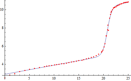
 I put the 0.1 x in manually -- Mathematica does not seem very good at finding the value for itself. Best, David
|
|
|
However I cannot alter the data, it's for a lab. Would it be logical to try to fit a sigmoid function (f(x)=a/(b+e^-x)) to the data? If so, how would I find and input the parameters? Thank you for your help on this matter
|
|
|
If I subtract about 0.1*x from each y the result looks much more like the usual logistic curve and the parameters for logistic might be easy to estimate.
|
|
|
Reply to this discussion
in reply to
|