Message Boards Message Boards

The Penrose tiling: casting night and day

Posted 2 years ago

Penrose Star Penrose Sun

In two previous posts on plane patterns, we discuss the relation between substitution systems, cellular automata and template atlases. Another plane pattern, the Penrose tiling, presents considerable difficulties in the form of non-crystallographic symmetry. Most people wouldn't bother to try and find a growth function, but we have two reasons to do just that. First, growth functions introduce a time variable, so provide a way from mathematical structure into physical process, thus toward the realm of quasicrystals. Second, perhaps more importantly, we would like to spend some of our limited time on this earth in the pursuit of pure beauty (even though pursuit of pure beauty might also be pursuit of total misery).

We need some functions to draw the actual tiles. To make the growth process easier, we put control points on every vertex, and allow for ten distinct orientations:

DepictThin[or_, v_, r_] := With[{verts = {{0, 0},
     {Cos[2 r Pi/10], Sin[2 r Pi/10]},
     {Cos[2 r Pi/10], Sin[2 r Pi/10]}
      + {Cos[2 (r - 1) Pi/10], Sin[2 (r - 1) Pi/10]},
     {Cos[2 (r - 1) Pi/10], Sin[2 (r - 1) Pi/10]}}},
  {White, Polygon[Expand@Plus[or, #, Part[-verts, v]] & /@ verts],
   Lighter@Red, 
   Disk[or + Part[-verts, v] + verts[[2]], 
    1/4, {2 (r - 1) Pi/10, 2 (r - 5) Pi/10}],
   Lighter@Purple, 
   Disk[or + Part[-verts, v] + verts[[4]], 
    1/4, {2 (r) Pi/10, 2 (r + 4) Pi/10}]}]

DepictFat[or_, v_, r_] := With[{verts = {{0, 0},
     {Cos[2 r Pi/10], Sin[2 r Pi/10]},
     {Cos[2 r Pi/10], Sin[2 r Pi/10]}
      + {Cos[2 (r - 2) Pi/10], Sin[2 (r - 2) Pi/10]},
     {Cos[2 (r - 2) Pi/10], Sin[2 (r - 2) Pi/10]}}},
  {White, Polygon[Expand@Plus[or, #, Part[-verts, v]] & /@ verts],
   Lighter@Purple, Disk[or + Part[-verts, v] + verts[[1]],
    1/4, {2 (r) Pi/10, 2 (r - 2) Pi/10}],
   Lighter@Red, Disk[or + Part[-verts, v] + verts[[3]],
    1, {2 (r + 5) Pi/10, 2 (r + 3) Pi/10}],
   White, Disk[or + Part[-verts, v] + verts[[3]],
    3/4, {2 (r + 5) Pi/10, 2 (r + 3) Pi/10}]}]
DepictRule = {TF -> DepictFat, TT -> DepictThin};

Fat and Thin

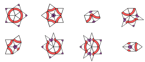
The one tile is usually called fat and the other thin. These tiles have matching rules, so they can only group around a vertex in one of eight legal vertex figures (in this case, vertex figures are essentially the same thing as what NKS calls templates). The atlas of all possible vertex figures is written out fully as:

Stars = Function[{off}, TF[{0, 0}, 1, 2 # - off] & /@ Range[5]] /@ {0,1};
Suns = Function[{off}, TF[{0, 0}, 3, 2 # - off] & /@ Range[5]] /@ {0, 1};
FHexes = Map[{TF[{0, 0}, 2, Mod[2 + #, 10]], 
     TF[{0, 0}, 4, Mod[4 + #, 10]],
     TT[{0, 0}, 2, Mod[5 + #, 10]]} &, Range[10]];
Crowns = Map[{TF[{0, 0}, 4, Mod[2 + #, 10]], 
     TF[{0, 0}, 2, Mod[4 + #, 10]],
     TT[{0, 0}, 3, Mod[4 + #, 10]], TF[{0, 0}, 3, Mod[3 + #, 10]],
     TT[{0, 0}, 1, Mod[6 + #, 10]]} &, Range[10]];
Boats = Map[{TF[{0, 0}, 1, Mod[6 + #, 10]], 
     TF[{0, 0}, 1, Mod[4 + #, 10]],
     TF[{0, 0}, 1, Mod[2 + #, 10]], TT[{0, 0}, 4, Mod[6 + #, 10]]} &, 
   Range[10]];
Splits = Map[{TF[{0, 0}, 3, Mod[#, 10]], TF[{0, 0}, 3, Mod[2 + #, 10]],
     TF[{0, 0}, 3, Mod[4 + #, 10]], TF[{0, 0}, 3, Mod[6 + #, 10]],
     TT[{0, 0}, 3, Mod[7 + #, 10]], TT[{0, 0}, 1, Mod[3 + #, 10]]} &, 
   Range[10]];
Wings = Map[{TT[{0, 0}, 1, Mod[7 + #, 10]], 
     TT[{0, 0}, 3, Mod[1 + #, 10]],
     TF[{0, 0}, 3, Mod[#, 10]],
     TT[{0, 0}, 1, Mod[3 + #, 10]], TT[{0, 0}, 3, Mod[7 + #, 10]],
     TF[{0, 0}, 3, Mod[6 + #, 10]], TF[{0, 0}, 3, Mod[4 + #, 10]]
     } &, Range[10]];
THexes = Map[{TT[{0, 0}, 4, Mod[#, 10]], TT[{0, 0}, 4, Mod[4 + #, 10]],
     TF[{0, 0}, 1, Mod[#, 10]]} &, Range[10]];
AllFigures = List[Suns, Stars, FHexes, Crowns, Boats, Splits, Wings, THexes];

Partition[Map[Graphics[{EdgeForm[Black], # /. DepictRule},
     PlotRange -> {{-2, 2}, {-2, 2}}, ImageSize -> 100] &,
   AllFigures[[All, 1]], {1}], 4] // TableForm

Penrose Vertices

Assume that we have a partially complete tiling and would like to add more tiles along the boundary. To do so, we need to know: which partial configurations have a unique completion? To answer this question, we simply calculate all possible partial configurations and notice when some are unique, while others project down from multiple vertex figures. The combinatorics can be programmed, so it ultimately requires very little thought:

FatEdges[or_, v_, r_] := With[{verts = {{0, 0},
     {Cos[2 r Pi/10], Sin[2 r Pi/10]},
     {Cos[2 r Pi/10], Sin[2 r Pi/10]}
      + {Cos[2 (r - 2) Pi/10], Sin[2 (r - 2) Pi/10]},
     {Cos[2 (r - 2) Pi/10], Sin[2 (r - 2) Pi/10]}}},
  Function[{verts},
    {FC[verts[[1]], Mod[r, 10]], TC[verts[[2]], Mod[r + 5, 10]],
     FC[verts[[1]], Mod[r - 2, 10]], TC[verts[[4]], Mod[r + 3, 10]],
     FR[verts[[4]], Mod[r, 10]], TR[verts[[3]], Mod[r + 5, 10]],
     FR[verts[[2]], Mod[r - 2, 10]], TR[verts[[3]], Mod[r + 3, 10]]}
    ][Expand@Plus[or, #, Part[-verts, v]] & /@ verts]]

ThinEdges[or_, v_, r_] := With[{verts = {{0, 0},
     {Cos[2 r Pi/10], Sin[2 r Pi/10]},
     {Cos[2 r Pi/10], Sin[2 r Pi/10]}
      + {Cos[2 (r - 1) Pi/10], Sin[2 (r - 1) Pi/10]},
     {Cos[2 (r - 1) Pi/10], Sin[2 (r - 1) Pi/10]}}},
  Function[{verts},
    {TR[verts[[1]], Mod[r, 10]], FR[verts[[2]], Mod[r + 5, 10]],
     TC[verts[[1]], Mod[r - 1, 10]], FC[verts[[4]], Mod[r + 4, 10]],
     FC[verts[[4]], Mod[r, 10]], TC[verts[[3]], Mod[r + 5, 10]],
     FR[verts[[2]], Mod[r - 1, 10]], TR[verts[[3]], Mod[r + 4, 10]]}
    ][Expand@Plus[or, #, Part[-verts, v]] & /@ verts]]

EdgesRule = {TF -> FatEdges, TT -> ThinEdges};

ProjectRules[figure_] := Rule @@ # & /@ Map[List[ Sort[
  Cases[figure[[1 ;; #]] /. EdgesRule, xF_[{0, 0}, yr_] :> xF[yr],
    Infinity]],
 figure[[#1 + 1 ;; -1]] ] &, Range[2, Length[figure] - 1]]

CompletionMap = Flatten[Map[Function[{rot}, ProjectRules[RotateRight[#, rot]]
     ] /@ Range[Length[#]] &, #] & /@ AllFigures];

UniqueCompletion = Cases[Tally[CompletionMap[[All, 1]]], {x_, 1} :> x];

UniqueMap = MapThread[ Rule, {UniqueCompletion, UniqueCompletion /. CompletionMap}];

AddRep[or_] := ReplaceAll[UniqueMap, {0, 0} -> or]

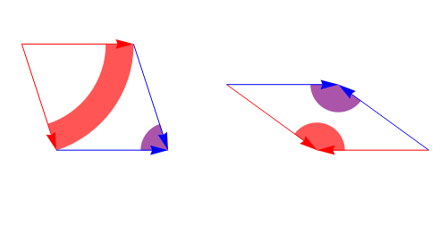
To see what we've done here (quite a lot by data structure and mapping), let's add another intermediary depiction function. There are $410$ total rules in AddRep, so we will only plot a random sample of 16:

DepictAddRule[rule_] := Show[Reverse[Map[Graphics[{EdgeForm[Thin],
       Arrowheads[.1], Thick, # /. DepictRule},
      ImageSize -> 150, PlotRange -> {{-2, 2}, {-2, 2}}] &, rule /. 
      Rule -> List /. {FR[r_] :> {Red, 
        Arrow[{{Cos[r Pi/5], Sin[r Pi/5]}, {0, 0}}]},
      FC[r_] :> {Blue, Arrow[{{Cos[r Pi/5], Sin[r Pi/5]}, {0, 0}}]},
      TR[r_] :> {Red, 
        Arrow[Reverse@{{Cos[r Pi/5], Sin[r Pi/5]}, {0, 0}}]},
      TC[r_] :> {Blue, 
        Arrow[Reverse@{{Cos[r Pi/5], Sin[r Pi/5]}, {0, 0}}]}}, 1]]]

Partition[DepictAddRule /@ RandomSample[AddRep[{0, 0}], 16], 
  4] // TableForm

update rules

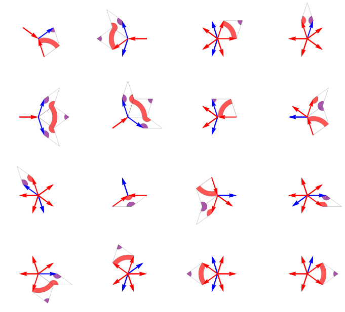
Basically, each image says that if we find this particular configuration of edge vectors in a partially complete tiling, then we should add one or more tiles, as depicted, to complete the figure. This is all good, but if we try to use only these $410$ rules, we quickly meet ambiguous conditions where we must choose one of two alternatives:

alternatives

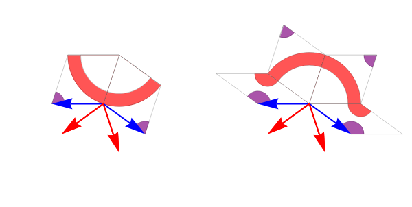
In another beautiful apparition of parity symmetry, it turns out the first alternative is better for growing the Night configuration, while the second is better for Day. All that's left is to define iterators and axioms as follows:

StarFailSafe[or_] := Join[
  Sort[{TC[Mod[2 + #, 10]], TC[Mod[6 + #, 10]], TR[Mod[3 + #, 10]], 
       TR[Mod[3 + #, 10]], TR[Mod[5 + #, 10]],
       TR[Mod[5 + #, 10]]}] -> {TF[or, 2, # + 1], 
      TF[or, 4, # - 1]} & /@ Range[10]]

SunFailSafe[or_] := Join[Sort[
      {TC[Mod[2 + #, 10]], TC[Mod[6 + #, 10]], TR[Mod[3 + #, 10]], 
       TR[Mod[3 + #, 10]], TR[Mod[5 + #, 10]],
       TR[Mod[5 + #, 10]]}] -> {TF[or, 3, # + 6], TF[or, 3, # + 4], 
      TT[or, 1, # - 3], TT[or, 3, # + 7]} & /@ Range[10],
  Sort[{TC[Mod[# + 1, 10]], TC[Mod[# + 1, 10]], TR[Mod[#, 10]], 
       TR[Mod[#, 10]],
       TR[Mod[# + 2, 10]], TR[Mod[# + 2, 10]], TR[Mod[# + 4, 10]], 
       TR[Mod[# + 8, 10]]
       }] -> {TF[or, 3, Mod[1 + #, 10]], 
      TF[or, 3, Mod[3 + #, 10]]} & /@ Range[10]]

CompleteFigures =   Map[Sort[Cases[# /. EdgesRule, xF_[{0, 0}, yr_] :> xF[yr], 
      Infinity]] &,   Flatten[AllFigures, 1]];

 IterateSunFS[state_, comp_] := With[{VertexFigures = Function[{edges},
      V[#, Sort[Cases[edges, x_[#, y_] :> x[y]]]] & /@ (
        Complement[Union[edges[[All, 1]]], comp])][
     Flatten[Union[state /. EdgesRule]]]},
  {Join[state, If[Length[#] == 0, Print["^"];
       With[{hits = 
          Cases[VertexFigures /. 
            V[or_, edges_] :> (edges /. SunFailSafe[or]), 
           TT[__] | TF[__], Infinity]},
        Sow[hits]; hits], #] &@
     Cases[VertexFigures /. V[or_, edges_] :> (edges /. AddRep[or]), 
      TT[__] | TF[__], Infinity]],
   Join[comp, 
    Cases[VertexFigures, 
     V[x_, Alternatives @@ CompleteFigures] :> x]]}]

IterateStarFS[state_, comp_] := With[{VertexFigures = Function[{edges},
      V[#, Sort[Cases[edges, x_[#, y_] :> x[y]]]] & /@ (
        Complement[Union[edges[[All, 1]]], comp])][
     Flatten[Union[state /. EdgesRule]]]},
  {Join[state, If[Length[#] == 0, Print["^"];
       With[{hits = 
          Cases[VertexFigures /. 
            V[or_, edges_] :> (edges /. StarFailSafe[or]), 
           TT[__] | TF[__], Infinity]},
        Sow[hits]; hits], #] &@
     Cases[VertexFigures /. V[or_, edges_] :> (edges /. AddRep[or]), 
      TT[__] | TF[__], Infinity]],
   Join[comp, 
    Cases[VertexFigures, 
     V[x_, Alternatives @@ CompleteFigures] :> x]]}]

AxiomA = TF[{0, 0}, 1, 2 #] & /@ Range[5];
StateA1 = {AxiomA, {{0, 0}}};
AxiomB = TF[{0, 0}, 3, 2 #] & /@ Range[5];
StateB1 = {AxiomB, {{0, 0}}};

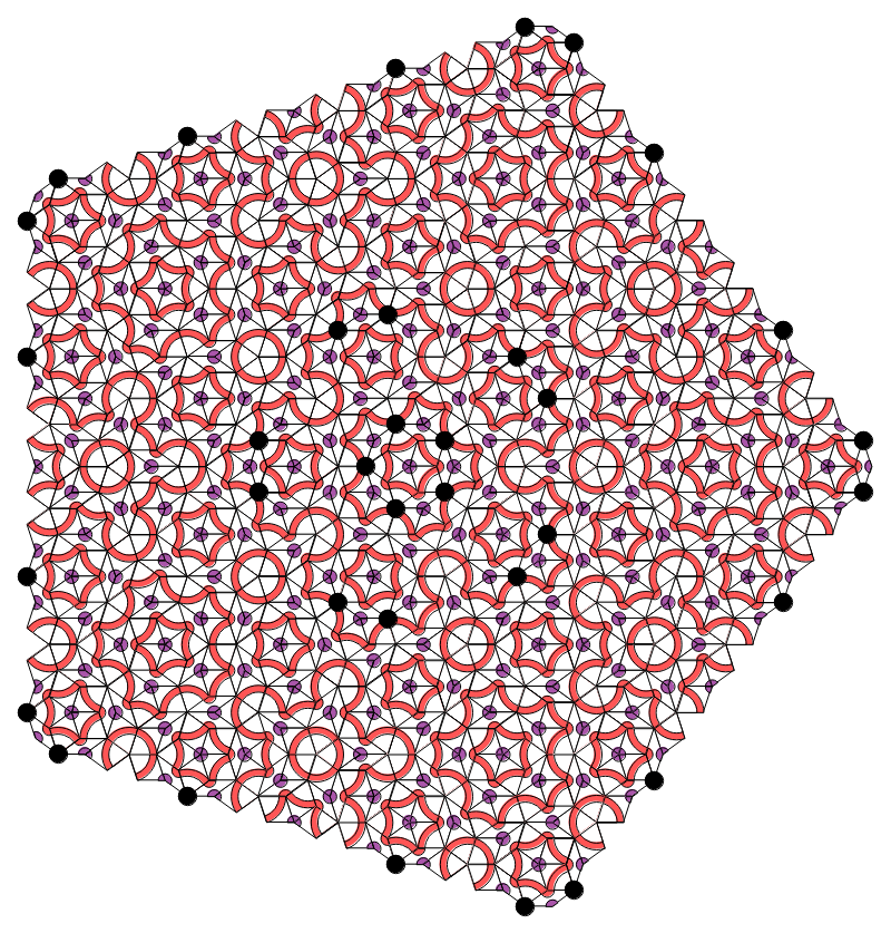
Now we can generate successive configurations and make a plot of where we were forced to make an arbitrary choice to continue growing the tiling. For the night configuration, we have, after about $35$ iterations:

AbsoluteTiming[ AData = Reap[NestList[IterateStarFS @@ # &, StateA1, 40]];]
Graphics[{EdgeForm[Black], AData[[1, -5, 1]] /. DepictRule, 
  Map[Disk[#, 1/3] &,   Union[Flatten[AData[[2, 1, All, All, 1]], 1]]]}, ImageSize -> 800]

ChoicesA

And for the Day configuration, we have, after about $45$ iterations:

AbsoluteTiming[ data = Reap[NestList[IterateSunFS @@ # &, StateB1, 50]];]

Graphics[{EdgeForm[Black], data[[1, -5, 1]] /. DepictRule, 
  Map[Disk[#, 1/3] &,
   Union[Flatten[data[[2, 1, All, All, 1]], 1]]]}, ImageSize -> 800]

Choices B

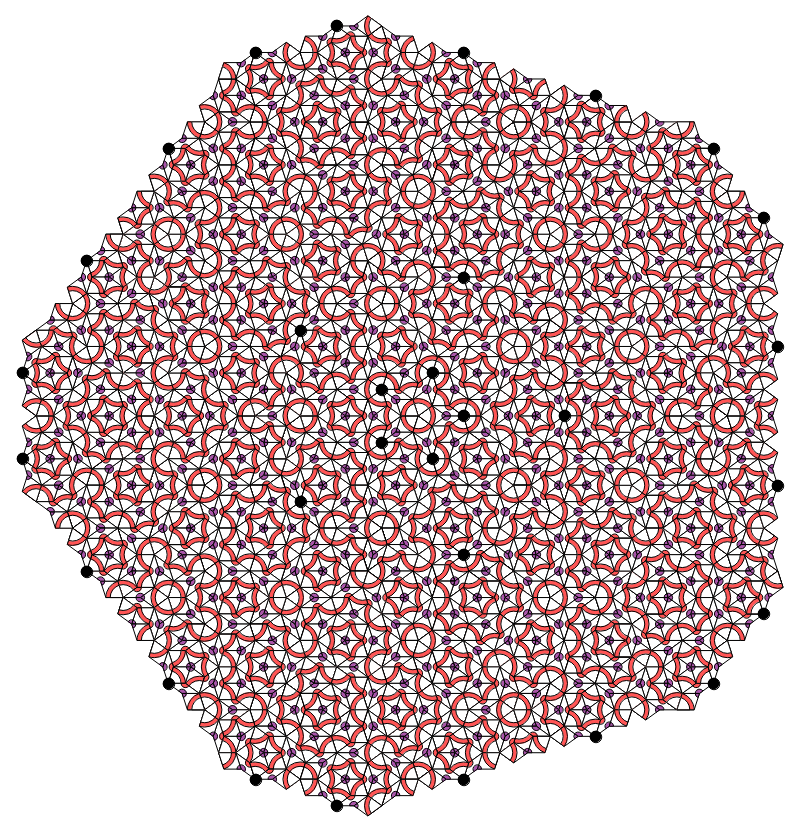
Using the same code, we can easily check both patterns up to $t\approx 150$, which gets us past the fourth or fifth wave / corona, in terms of light-red loops drawn around the pattern center. This very strongly suggests that the algorithm as presented here will grow patterns indefinitely. However, a little more work remains to be done to make the algorithm a proper Cellular Automaton algorithm. This can likely be accomplished by adding an extra binary variable at all binary-ambiguous vertices. This project we leave for another day...

POSTED BY: Brad Klee
6 Replies

Hey thanks!

Penrose triality pattern

Here's one more graph: Growing the Penrose tiling Triality pattern. Adding one of three colors to star-centers ultimately decides all binary choices. The two alternate vertex configurations do not occur in equal proportion, and the above graph marks the less frequent figure in lime green. A very nice feature of this pattern is that all green vertices fall on a thick edge of one of the three or four larger tiles. After about ~100 time steps, we have:

bigger pic

So yes, it appears the Penrose tiling can be grown by a deterministic local rule, but the neighborhood may need to be on distance scale $\phi^4$ (as seen in the background).

POSTED BY: Brad Klee

It appears that slight modification of the growth rules allows for synchronization of star-center turn-ons. This looks to be leading toward verification of a log-periodic Ulam Structure: at times $t = k^n, n \in 1, 2, \ldots$ the growth function goes extinct except for singular sources at each of five pentagonal corners (which alternate between even / odd $D_{10}$ axes as $n$ increases). The following animation goes through $n=1$ and $n=2$ with only a few sync errors:

Fractal Penrose

POSTED BY: Brad Klee

Fully Synchronized Penrose Tiling

Synchronization is important to long range order, since it can effectively prevent patterns of destructive interference from introducing wrong configurations. While mathematically perfect growth functions may not ever occur in the quasicrystal lab, they can certainly give us insight to what may happen there. The biggest takeaway (which is hinted at in Socolar's "Growth Rules for Quasicrystals") is that frustration is an important part of growing Ulam structures. Snowflakes tend to grow on corners due to sharpness of the electromagnetic field, so perhaps a similar mechanism affects quasicrystals.

Now that we have a perfectly synchronized function up to time $t \sim 100$, we can calculate the growth sequences fairly easily:

Length /@ AStates[[All, 2, 2]]
Differences[%]
Divide[%% - 1, 5]
Divide[%%, 5]
Transpose[Partition[%, 4]]

(* editor's note: these sequences have been corrected on Oct. 26 *)
Out[]:= {1, 1, 1, 1, 1, 6, 6, 6, 6, 16, 16, 16, 16, 21, 21, 21, 21, 36, 36, 
36, 36, 61, 61, 61, 61, 71, 71, 71, 71, 101, 101, 101, 101, 121, 121, 
121, 121, 136, 136, 136, 136, 156, 156, 156, 156, 176, 176, 176, 176, 
191, 191, 191, 191, 236, 236, 236, 236, 306, 306, 306, 306, 331, 331, 
331, 331, 396, 396, 396, 396, 441, 441, 441, 441, 471, 471, 471, 471, 
511, 511, 511, 511, 551, 551, 551, 551, 581, 581, 581, 581, 671, 671, 
671, 671, 736, 736, 736, 736, 751, 751, 756}
Out[]:= {0, 0, 0, 0, 5, 0, 0, 0, 10, 0, 0, 0, 5, 0, 0, 0, 15, 0, 0, 0, 25, 0, 
0, 0, 10, 0, 0, 0, 30, 0, 0, 0, 20, 0, 0, 0, 15, 0, 0, 0, 20, 0, 0, 
0, 20, 0, 0, 0, 15, 0, 0, 0, 45, 0, 0, 0, 70, 0, 0, 0, 25, 0, 0, 0, 
65, 0, 0, 0, 45, 0, 0, 0, 30, 0, 0, 0, 40, 0, 0, 0, 40, 0, 0, 0, 30, 
0, 0, 0, 90, 0, 0, 0, 65, 0, 0, 0, 15, 0, 5} (* note sync breaking *)
Out[]:= {0, 0, 0, 0, 0, 1, 1, 1, 1, 3, 3, 3, 3, 4, 4, 4, 4, 7, 7, 7, 7, 12, 
12, 12, 12, 14, 14, 14, 14, 20, 20, 20, 20, 24, 24, 24, 24, 27, 27, 
27, 27, 31, 31, 31, 31, 35, 35, 35, 35, 38, 38, 38, 38, 47, 47, 47, 
47, 61, 61, 61, 61, 66, 66, 66, 66, 79, 79, 79, 79, 88, 88, 88, 88, 
94, 94, 94, 94, 102, 102, 102, 102, 110, 110, 110, 110, 116, 116, 
116, 116, 134, 134, 134, 134, 147, 147, 147, 147, 150, 150, 151}
Out[]:={0, 0, 0, 0, 1, 0, 0, 0, 2, 0, 0, 0, 1, 0, 0, 0, 3, 0, 0, 0, 5, 0, 0, 
0, 2, 0, 0, 0, 6, 0, 0, 0, 4, 0, 0, 0, 3, 0, 0, 0, 4, 0, 0, 0, 4, 0, 
0, 0, 3, 0, 0, 0, 9, 0, 0, 0, 14, 0, 0, 0, 5, 0, 0, 0, 13, 0, 0, 0, 
9, 0, 0, 0, 6, 0, 0, 0, 8, 0, 0, 0, 8, 0, 0, 0, 6, 0, 0, 0, 18, 0, 0, 
0, 13, 0, 0, 0, 3, 0, 1}
Out[]:= {
{0, 1, 2, 1, 3, 5, 2, 6, 4, 3, 4, 4, 3, 9, 14, 5, 13, 9, 6, 8, 8, 6, 18, 13}, 
{0, 0, 0, 0, 0, 0, 0, 0, 0, 0, 0, 0, 0, 0, 0, 0, 0, 0, 0, 0, 0, 0, 0, 0}, 
{0, 0, 0, 0, 0, 0, 0, 0, 0, 0, 0, 0, 0, 0, 0, 0, 0, 0, 0, 0, 0, 0, 0, 0}, 
{0, 0, 0, 0, 0, 0, 0, 0, 0, 0, 0, 0, 0, 0, 0, 0, 0, 0, 0, 0, 0, 0, 0, 0}}

The first sequence is the number of suns turned on at time $t$. None of these integer sequences appear to be on OEIS, though many similar sequences are. Actually, the growth algorithm is fairly difficult to program, so it's more likely that OEIS would have something on the triality pattern itself, for example:

Length /@ NestList[Function[{verts}, Union@Join[Flatten[
      Nearest[Complement[AStates[[-1, 2, 2]] , verts ], #] & /@ verts,
       1], verts]], {{0, 0}}, 10]
Divide[% - 1, 5]
Differences[%]
Differences[%%%]

Out[276]= {1, 6, 16, 21, 36, 61, 81, 106, 136, 176, 211}
Out[277]= {0, 1, 3, 4, 7, 12, 16, 21, 27, 35, 42}
Out[278]= {1, 2, 1, 3, 5, 4, 5, 6, 8, 7}
Out[279]= {5, 10, 5, 15, 25, 20, 25, 30, 40, 35}

Neither do any of these appear in OEIS, so perhaps we are really doing something fun and original here.

POSTED BY: Brad Klee

combined grow

After correcting an error in the above process, I decided to double check using an entirely different algorithm. The new technique (still under development) does not use tiles, but instead grows the triality pattern directly by adding branches at each successive iteration. This process produces a slightly different count:

Length[Union[Flatten[#][[All, 1]]]] & /@ stateList[[1 ;; 24]]
Differences[%]/5
Subtract[%, {1, 2, 1, 3, 5, 2, 6, 4, 3, 4, 4, 3, 9, 14, 5, 13, 9, 6, 8, 8, 6, 18, 13}]

Out[]:= {1, 6, 16, 21, 36, 61, 71, 101, 131, 146, 156, 176, 191, 236, 306,
331, 396, 461, 491, 511, 551, 581, 671, 771}
Out[]:={1, 2, 1, 3, 5, 2, 6, 6, 3, 2, 4, 3, 9, 14, 5, 13, 13, 6, 4, 8, 6, 18, 20}
Out[]:={0, 0, 0, 0, 0, 0, 0, 2, 0, -2, 0, 0, 0, 0, 0, 0, 4, 0, -4, 0, 0, 0,7}

At some times, the branching algorithm grows slightly faster than the tiling algorithm, which then catches up after two steps.

The agreement of these result is very exciting, but minor disagreements show that we still don't know exactly how to define the growth sequence. The growth algorithm runs smoothly up to about $t \sim 45$, and then we may need to rethink conditional rules. We'll see what happens soon...

POSTED BY: Brad Klee

Another definition of the triality pattern is that it is the Original Penrose Tiling if you leave out stars and partial stars, taking the pentagons only, in three colors, according to neighbors. See for example, this picture on wikipedia.

In continuing to explore branching algorithms, I produced the following animations by means of a relatively simple algorithm:

Day Growth

Night Growth

Here "relatively simple" still means "quite complex", and as written, the algorithm may not be entirely complete. In one run to time $t=500$, I noticed a hole:

sun500 star500 (zoom in if possible)

However, we can check that holes can be correctly filled by looking at overlap with the ambient green pattern. The night and day duality should require five gray pentagons to fall in every green pentagon. From quick perusal this appears to be the case, even on the front, which is still growing wherever vertices are blue. Probably what's happened is that one of the case tables is incomplete. Later that sort of error can be corrected by fine tuning.

At such an advanced stage, it becomes difficult to perform quality analysis other than sitting back to watch and appreciate the animation. However, we can print out statistics about the growth, including count of new vertexes added, for example:

data=CountDifferences[StateList]
Total[%]
ListPlot[%%]
Out[]:={1, 2, 1, 3, 5, 2, 6, 4, 1, 4, 6, 3, 9, 14, 5, 13, 9, 2, 8, 12, 6, 
18, 14, 4, 11, 8, 3, 3, 6, 4, 12, 15, 6, 18, 11, 3, 12, 18, 9, 27, 
38, 14, 38, 25, 5, 18, 26, 13, 39, 32, 9, 23, 17, 7, 7, 16, 8, 24, 
30, 12, 36, 22, 6, 24, 36, 18, 54, 44, 15, 38, 32, 6, 13, 20, 11, 33, 
26, 9, 14, 12, 6, 9, 10, 3, 9, 14, 6, 18, 13, 4, 16, 24, 12, 36, 44, 
15, 39, 26, 6, 24, 36, 18, 54, 38, 11, 32, 20, 9, 9, 18, 12, 36, 45, 
18, 54, 33, 9, 36, 54, 27, 81, 106, 38, 102, 67, 14, 52, 76, 38, 114, 
84, 24, 65, 46, 17, 15, 34, 18, 54, 65, 26, 78, 47, 13, 52, 78, 39, 
117, 98, 34, 88, 71, 13, 28, 42, 23, 69, 56, 19, 29, 25, 12, 21, 20, 
9, 21, 34, 16, 48, 29, 8, 32, 48, 24, 72, 88, 30, 78, 52, 12, 48, 72, 
36, 108, 76, 22, 64, 40, 18, 18, 36, 24, 72, 90, 36, 108, 66, 18, 72, 
108, 54, 162, 148, 48, 119, 88, 17, 55, 78, 42, 114, 90, 32, 80, 47, 
16, 17, 28, 17, 43, 65, 36, 70, 46, 27, 48, 90, 39, 83, 86, 39, 71, 
51, 24, 30, 50, 30, 46, 54, 18, 29, 22, 8, 19, 20, 11, 27, 25, 10, 
30, 12, 3, 12, 18, 9, 27, 38, 14, 38, 25, 6, 24, 36, 18, 54, 42, 13, 
37, 28, 12, 12, 24, 16, 48, 60, 24, 72, 44, 12, 48, 72, 36, 108, 120, 
42, 114, 74, 15, 54, 78, 39, 117, 92, 26, 68, 47, 21, 21, 48, 24, 72, 
90, 36, 108, 66, 18, 72, 108, 54, 162, 116, 37, 90, 80, 17, 37, 54, 
32, 84, 72, 31, 58, 37, 17, 26, 26, 9, 27, 42, 18, 54, 39, 12, 48, 
72, 36, 108, 124, 41, 105, 70, 16, 64, 96, 48, 144, 104, 31, 90, 60, 
27, 27, 54, 36, 108, 127, 50, 150, 91, 25, 100, 150, 75, 225, 290, 
104, 280, 183, 38, 140, 204, 102, 306, 228, 65, 175, 122, 48, 44, 
100, 52, 156, 190, 76, 228, 138, 38, 152, 228, 114, 342, 268, 90, 
227, 192, 38, 75, 116, 65, 195, 150, 51, 76, 64, 30, 50, 49, 22, 44, 
74, 37, 98, 66, 28, 70, 114, 64, 149, 189, 68, 158, 112, 36, 102, 
162, 82, 219, 162, 48, 131, 83, 42, 40, 84, 63, 150, 198, 83, 219, 
144, 54, 153, 243, 138, 334, 322, 113, 242, 192, 58, 122, 192, 104, 
233, 195, 77, 168, 96, 33, 35, 60, 38, 82, 131, 72, 134, 89, 53, 92, 
174, 75, 157, 162, 74, 130, 95, 48, 64, 108, 64, 104, 114, 39, 70, 
56, 25, 47, 54, 32, 84, 72, 27, 64, 31, 13, 40, 48, 25, 69, 100} 

Out[]:=30216 

Ulam Structure

This graph strongly indicates that the Ulam structure has been achieved, since it returns log-periodically to minimum values $3$ and $6$:

Flatten[Position[data, 3]]
%*3
{4, 12, 27, 28, 36, 84, 252}
{12, 36, 81, 84, 108, 252, 756}

Flatten[Position[data, 6]]
%*3
Out[]={7, 11, 21, 29, 33, 63, 72, 81, 87, 99, 261}
Out[]={21, 33, 63, 87, 99, 189, 216, 243, 261, 297, 783}

We can almost begin to form a hypothesis about recurrence of local minima in the count function, but we are also worried about rigor. Although this function (assuming it can be finalized and fully debugged) appears to be complete and to have the Ulam structure, these properties need to be proven. Additionally, more work needs to be done to prove that the growth function can be fully localized. (For now I can only give a hint: The new growth rule depends on three look-back functions: One to decide branching off black, one to decide odd-angle Gray $+$ Gray $\rightarrow $ White, and one to decide Gray $\rightarrow$ White on star fronts. Other than those three caveats, it is also a local, cellular-automaton-style growth rule.)

Comparing with Socolar's 1991 algorithm from Growth Rules for Quasicrystals, our candidate features synchronized and deterministic growth. One physical question is whether or not synchronization of growth on near fronts helps to establish long range aperiodic order?

Thanks for your time and numerous likes.

--Brad

POSTED BY: Brad Klee

enter image description here -- you have earned Featured Contributor Badge enter image description here Your exceptional post has been selected for our editorial column Staff Picks http://wolfr.am/StaffPicks and Your Profile is now distinguished by a Featured Contributor Badge and is displayed on the Featured Contributor Board. Thank you!

POSTED BY: Moderation Team
Reply to this discussion
Community posts can be styled and formatted using the Markdown syntax.
Reply Preview
Attachments
Remove
or Discard

Group Abstract Group Abstract