Thanks for your response to the Print issue I posted. The CellPrint code you provided works well. Based on that, I went back to the Print Help. My take on that is that Print generates something like CellPrint, though my attempt to use FullForm[HoldForm[Print[...]]] did not work. How does one find what the underlying Wolfram Language code of Print is or is Print just a function unto itself? That is, how do I find out whether Print is using CellPrint? Since Print has no options, I tried Grid with Frame -> True, which shows that the width is set to that of the wider of the two lines of text. This suggests that at least part of the Print problem may have to do with cell width being set this way. To fix this, I added to Grid the option ItemSize. Here is the code, which works fine:
Grid[{{Style["Options for Plot and ListPlot", Bold, 16,
Orange]}, {Style["Options in Common", Italic, 14, Blue]}},
Alignment -> Center, Frame -> True, ItemSize -> 50]
Attached file "GDorfman_GridToCenterText.nb" has the above code with and without ItemSize along with the corresponding output.
 Attachments:
|
|
|
If you create DockedCells eg  How do you remove it ?
|
|
|
Doug, To remove all docked cells
SetOptions[EvaluationNotebook[], DockedCells -> {}]
|
|
|
Input
NRoots[x^2 == 5, x] gives me an error:
... General: 5 is not a valid variable. What's wrong?
|
|
|
Try evaluating x by itself and I think you'll see where the Irishman comes from :). Run ClearAll[x] after that and NRoots will do its job as expected.
|
|
|
I was delighted to learn how fancy Mathematica is regarding integrating over regions. Yesterday's lecture (April 28, 2022) illustrated some really cool things that got me excited. I played around with some examples, for the fun of it. This is a really nice ability. I am including the notebook with 2 neat examples. Oddly there might be a bug, although the "bug" is probably mine. It is amazing that one can integrate over such exotic regions. See the attached notebook.
Attachments:
|
|
|
I feel like I am doing something exceedingly stupid, but am having trouble getting the volume of a sphere as given below. 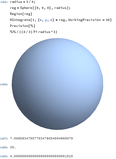
This calculation gives 7.06858347057703478654094869079, which is off by a factor of 4.
|
|
|
Try Ball instead of Sphere—despite colloquial usage, a sphere is a 2D object that embeds into 3D space.
|
|
|
Arben, thank you for your kind response. Indeed, the use of Ball in place of Sphere makes everything work wonderfully.
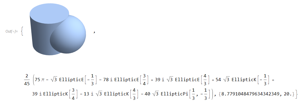
I went on to play around with some cool and fun examples, and I am including the updated notebook.
Here is a highlighted example from the attached notebook, where it finds a closed form solution.
Attachments:
|
|
|
I'm glad to hear it! I might be biased, but I do think it's pretty cool that you're able to achieve such a result. Also—while this may be a bit trivializing in some sense, we really do have a function for everything! Try out RegionMeasure, if you'd like, e.g.:
Manipulate[
 RegionMeasure /@ {Disk[{0, 0}, d], Sphere[{0, 0, 0}, d],
   Ball[{0, 0, 0}, d], Cuboid[{0, 0, 0}, d {1, 1, 1}]}, {d, 1, 5, 1}]
This can be useful to provide some insight which is relevant to the dimensionality question we're discussing (somewhat paradoxically). On a related note, you might try something like Volume[Sphere[]] and get a (previously-)surprising result. Or, you could make the variation continuous, then Plot to see the problem another way:
Plot[Evaluate[
  RegionMeasure /@ {Disk[{0, 0}, d], Sphere[{0, 0, 0}, d],
    Ball[{0, 0, 0}, d], Cuboid[{0, 0, 0}, d {1, 1, 1}]}], {d, 1, 5},
 ScalingFunctions -> {"Log", "Log"}]
(adding PlotLegends->"Expressions" would make it explicit, to wit.) EDIT: I'd be loathe to forget RegionDimension!
|
|
|
Arben, thank you for your additional comments (BTW, which were made on a Saturday), which I am now beginning to work on. I wanted to dash off a quick note as I am just up on this Sunday and have just taken the first sip of coffee. To wit: I am more than biased regarding Mathematica. I am dazzled by the cool things that you can do with it. It is amazing that one can measure the volume of such incredible regions in 3-space. It is amazing that it finds a closed form solution in terms of elliptic functions for one of the volumes in my last note. This also works in 4-space and more. Recently, following the documentation, I did an integral in 1000 dimensions. (An interesting problem is defining the integrand here.) It is not unusual for me to spend hours, sometimes more than 12, "just" studying the documentation. Mathematica does so many amazing things. I am going to play around with RegionMeasure some, as you suggested. I am sure it is a much better implementation than my own regionIntegrate3D (see included notebook) that I had concocted just to play around, to practice, to hone skills, etc. I note that this is recreational mathematics. I am doing this for fun, but also hope it might lead to something wonderful. My apologies for not being better than I am at Mathematica: I have loved it since VERSION ONE (circa 1987 or so). For someone who has used it a long time, I should be better at it. I am spread very thin pursuing many interests, especially including music and photography. To play around with (tagged) upvalues, I might try to play with a concept similar to the class example "n g[x] expanding to g[n x]". While laying in bed this morning, I thought about something like 3 h[Ball[]] creating 3 balls. This can generalize nicely. If it sees n g[x] as a pattern, maybe it will see {point1,point2,n} * h[Ball[]] as an upvalue for h, and then construct n Balls from point1 to point2, but only if the symbol h is used. This is just fantasy (fantasia) now, but I might want to play around with this.
|
|
|
Additional notes on this comment from above.
"If it sees n g[x] as a pattern, maybe it will see {point1,point2,n} *
h[Ball[]] as an upvalue for h, and then construct n Balls from point1
to point2, but only if the symbol h is used."
I want to create a simple "extension" using tagged delayed assignments (up values) to allow n points to be enumerated over a line from point1 to point2.
We try this naively and find that the implicit multiply operation is listable, so we get a list of the multiplied values.
In[150]:= ClearAll[g]
g /: n_List g[x_] := g2[g1[n], x]
{point1, point2, n} g[x]

Out[152]= {point1 g[x], point2 g[x], n g[x]}
This is not what we want. Instead of using the Times[] function, we will use h, which is not listable, in the above instead.
In[144]:= ClearAll[g]
g /: h[n_List, g[x_]] := g2[g1[n], x]
h[{point1, point2, n}, g[x]]

Out[146]= g2[g1[{point1, point2, n}], x]
g1 can be a function to generate the n points and then it is passed to g2 which does the volume rendering of x. Maybe there is an existing function for this, but this is a fun exercise anyway. Basically, we are recognizing a certain context involving an outer scope of the function g, and then doing something special to it when we recognize it. This is an amazing ability! WOW! I learned a lot in writing this stuff up. Tagged delayed assignments are really cool, and I had fun playing with the concepts which I had just recently learned.
|
|
|
I am adding to the ""If it sees n g[x] as a pattern" from above. Using a tagged delayed assignment to generate a list of volumes along a lineTwo relatively simple lines of code make it easy to generate volume objects along a straight line.
LinePoints[{p1_, p2_, n_}] := Table[p1 + (p2 - p1) k/n, {k, 0, n}];
UsingA /: GenerateLinearRegion[n_List, UsingA[x_]] :=
 Region[RegionUnion[Map[x[#] &, LinePoints[n]]]]
Here UsingA is a tagged delayed assignment. Its use makes it easy to generate volumes. For example
GenerateLinearRegion[{{0, 5, 0}, {15, 0, 0}, 10}, UsingA[Ball]]
generates a series of 11 Ball objects from {0,5,0} to {15,0,0}, and is shown below. 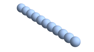
Another example is here. 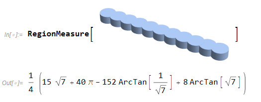
A more complex structure is also easy to generate. 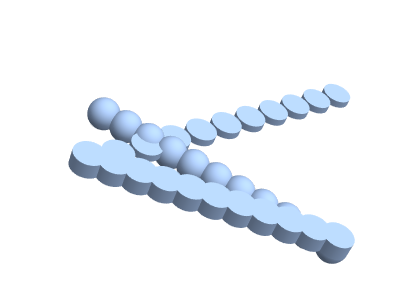
These examples are from the attached notebook, which includes more illustrations. The tagged delayed assignment is a really cool feature of WL.
Attachments:
|
|
|
Attachments:
|
|
|
I am repeating this calculation using RegionMeasure. It is totally amazing that Mathematica finds a closed form solution!!! Don't complain if it takes a few minutes -- wanna try it by hand?? haha. 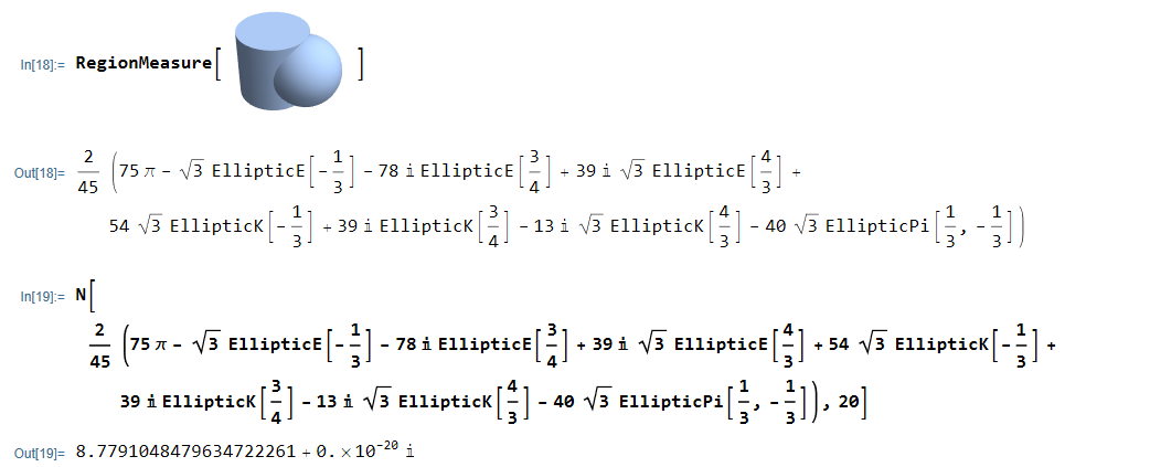
|
|
|
Expanding on your comments, Arben, we see indeed that integrating using Sphere vs. Ball clearly gives different answers.
In[6]:= Integrate[1, {x, y, z} \[Element] Sphere[]]

Out[6]= 4 \[Pi]

In[7]:= Integrate[1, {x, y, z} \[Element] Ball[]]

Out[7]= (4 \[Pi])/3
Using RegionMeasure allows the dimension of the integration to be specified.
In[8]:= RegionMeasure[Sphere[]]

Out[8]= 4 \[Pi]
Agreeing with your comment, Arben, Sphere[] is 2-dimsional, and its 3-D measure gives zero. WOW - that's a gocha.
In[10]:= RegionMeasure[Sphere[], 3]

Out[10]= 0
Note the correct answers using Ball[] below.
In[9]:= RegionMeasure[Ball[]]

Out[9]= (4 \[Pi])/3

In[11]:= RegionMeasure[Ball[], 3]

Out[11]= (4 \[Pi])/3
As a final note, we see and understand the next result.
In[12]:= RegionMeasure[Ball[], 4]

Out[12]= 0
|
|
|
More comments regarding Ball and SphereI am not claiming that there is an error here, only just misuse and misunderstanding (by me) of an understandably tricky point. We have the same issue regarding Circle[] and Disk[]. Circle is the 1 dimensional circle (circumference) whereas Disk[] is the filled 2 dimensional object.
We see this in the following three calculations. The circumference of the unit circle is 2 Pi.
In[121]:= RegionMeasure[Circle[]]

Out[121]= 2 \[Pi]

In[124]:= RegionMeasure[Circle[], 1]

Out[124]= 2 \[Pi]

In[122]:= RegionMeasure[Circle[], 2]

Out[122]= 0

In[123]:= RegionMeasure[Disk[], 2]

Out[123]= \[Pi]
Now, with Disk[] we find the area of the unit circle or Pi. These results all make sense. We have a similar situation regarding Sphere[] and Ball[]. The RegionMeasure of the Sphere[] is its 2-dimsional surface area, which is 4 Pi, whereas the RegionMeasure of Ball[] is its 3-dimensional volume, which is 4 Pi/3.
In[126]:= RegionMeasure[Sphere[], 2]

Out[126]= 4 \[Pi]

In[127]:= RegionMeasure[Sphere[], 3]

Out[127]= 0

In[128]:= RegionMeasure[Ball[], 3]

Out[128]= (4 \[Pi])/3
This all makes sense, now, but this is an easy point to get tripped up over. Arben, thanks for bringing this to light!
Clearly, this is not an error, and it should be this way, but this is definitely a very subtle point.
|
|
|
Looking for a possible application for upvalues, I made the following definition:
f[x_ /; x < 1] := 1;

f[x_ /; x >= 1] := x x x;

Sqrt[f[x_] /; x >= -2 && x <= -1 ] ^:= 3;
If I now want to test the effectiveness of my definition by calculating a square root of f[-1.5], it does not seem to work at first glance:
Sqrt[ f[-1.5]] returns 1, and not the expected 3.
The same applies to a function plot:
Plot[Sqrt[ f[x]], {x, -5, 5} ]
On closer analysis, it turns out that the calculation first calculates the inner term, and the kernel then forgets that the inner value arose by evaluating f[x], and accordingly does not apply the upvalue. If I forbid the evaluation of the inner term, we get the expected results:
Sqrt[ Unevaluated[ f[-1.5]]]

Plot[Sqrt[ Unevaluated[f[x]]], {x, -5, 5} ]
This shows me that upvalues do not allow the overloading of functions similar to OOP that I had hoped for. Always thinking about disallowing the evaluation of the inner term limits the usability in my eyes. However, this begs the question. What is a real life use case for the upvalues?
|
|
|
@Peter Lippolt here is an explanation from the instructor Dave Withoff
The essential issue raised by the example
In[]:= f[x_ /; x < 1] := 1
In[]:= f[x_ /; x >= 1] := x x x
In[]:= Sqrt[f[x_] /; x >= -2 && x <= -1] ^:= 3

In[]:= Sqrt[f[-1.5]]
Out[]= 1
is the question of what the system should do when two rules apply to
the same input, rather than a specific feature of upvalues. The problem is that the rule for f[x_ /; x < 1] and the rule for
Sqrt[f[x_] /; x >= -2 && x <= -1] both apply to Sqrt[f[-1.5]]. Without
further information, the computer has no way of knowing which rule to
use. In the Wolfram Language, the default, following the principle of
standard order evaluation (evaluating the elements of an expression
before evaluating the enclosing expression), is to evaluate f[-1.5],
which has the effect of applying the rule for f[x_ /; x < 1]. There are many ways to get the rules applied in a different order. One
method is to enter all of the rules as upvalues for f:
In[]:= Sqrt[f[x_] /; x >= -2 && x <= -1] ^:= 3
In[]:= f /: _[f[x_ /; x < 1]] := 1
In[]:= f /: _[f[x_ /; x >= 1]] := x x x

In[]:= Sqrt[f[-1.5]]
Out[]= 3
Entering all of the rules as upvalues like this is closer conceptually
to the way this would work in an OOP system. Mixing upvalues and
downvalues potentially increases confusion about which will be used
first. A few observations about this behavior: 1) Comparable issues will arise in any system, including OOP systems.
If two rules, or two methods, apply in the same situation, the
computer has to somehow resolve the conflict. Different systems will
handle the conflict in different ways, but the conflict will remain. 2) Conflicts like this are rare in practical applications. It is easy
to make up examples where the system is presented with ambiguous
instructions and has to follow some default or some process for
deciding what to do, but in practical applications such ambiguities
usually either don't come up in the first place, or are resolved in
some other way. 3) To address the question about real-life uses of upvalues, there are
a number of large applications of upvalues. Two prominent examples are
the rules for series expansions, and implementation of non-commutative
algebra. The built-in rules for series expansions are implemented as upvalues
for SeriesData. SeriesData is the symbol that is used for representing
series expansions. For convenience of programming, the rules for
series expansions are implemented as upvalues for SeriesData rather
than as downvalues for individual functions. For example, Series[Exp[x], {x, 0, 3}] is evaluated by first
constructing SeriesData[x, 0, {1}, 1, 4, 1], which is the series
expansion to degree 3 for x by itself, and then applying Exp to that
SeriesData expression. The result is normally formatted as a sum, but
the SeriesData expression can be seen using InputForm:
In[]:= Exp[SeriesData[x, 0, {1}, 1, 4, 1]] // InputForm

Out[]//InputForm= SeriesData[x, 0, {1, 1, 1/2, 1/6}, 0, 4, 1]
The rules that gave that result, and the rules for doing series
expansions of other functions, are implemented as upvalues for
SeriesData. Comparable rules could be entered as downvalues for
individual functions, such as the Exp function, but it is easier to do
the programming if all of the rules for series expansions are in one
place, attached to SeriesData, rather than scattered throughout the
system among all of the other rules for individual functions. Similarly, it is convenient when entering rules for non-commutative
algebra to attach rules as upvalues for elements of the algebra. For
example, using the ** notation for NonCommutativeMultiply:
In[]:= x /: x[p_] ** x[q_] := -x[q] ** x[p] /; ! OrderedQ[{p, q}]

In[]:= x[2] ** x[1]

Out[]= -x[1] ** x[2]
A comparable rule could have been entered by unprotecting the built-in
symbol NonCommutativeMultiply and entering a downvalue for
NonCommutativeMultiply, but some consider it easier or more natural to
instead enter a rule like this as upvalue for x.
|
|
|
The first two Print statements below center the text. The third Print statement, which just combines the first two, does not center the text. Attached file "GDorfman_PrintIssue.nb" shows the three Print statements and their output. Why does the third Print statement not center the text? How can it be modified so it does center the text?
Print[Style["Options for Plot and ListPlot",Bold,16,Orange,TextAlignment->Center]]

Print[Style["\nOptions in Common\n",Italic,14,Blue,TextAlignment->Center]]

Print[Style["Options for Plot and ListPlot",Bold,16,Orange,TextAlignment->Center],
Style["\nOptions in Common\n",Italic,14,Blue,TextAlignment->Center]]
Attachments:
|
|
|
The documentation for Print says:
- Print[Subscript[expr, 1],Subscript[expr, 2],[Ellipsis]] prints Subscript[expr, i] concatenated together, effectively using Row
- You can arrange to have expressions on several lines by using Column.
So the output I see is the same as what the following provides:
Row[{
  Style["Options for Plot and ListPlot", Bold, 16, Orange, TextAlignment -> Center],
  Style["\nOptions in Common\n", Italic, 14, Blue, TextAlignment -> Center]
  }, Alignment -> Right]
The Alignment option does not quite center the output within the output cell.
The best I could come up with was:
Print[
 Column[{
   Style["Options for Plot and ListPlot", Bold, 16, Orange,
    TextAlignment -> Center],
   Style["\nOptions in Common\n", Italic, 14, Blue,
    TextAlignment -> Center]
   }, Alignment -> Center]
 ]
Even this does not produce the output that you probably want. However with Print ultimately creating a "cell", I wondered why not just use CellPrint that is supposed to insert a cell in the current notebook. So here is what I have:
CellPrint[
 {
  TextCell[Style["Options for Plot and ListPlot", "Output", Bold, 16, Orange, TextAlignment -> Center]],
  TextCell[Style["Options in Common", "Output", Italic, 14, Blue, TextAlignment -> Center]]
  }
 ]
This output seems more like what you want to see.
|
|
|
[WSG22] Daily Study Group: A Guide to Programming and Mathematics with WL
|
|
|
The notebook for Friday's lesson (#19) appears to be missing. When will it be made available?
|
|
|
Notebook 19SolvingEquations.nb has now been added.
|
|
|
Is there a way to prevent Mathematica from inserting spaces into a URL I put in a notebook? If I copy a URL into Mathematica, then copy it from there, it comes out like this: https : // www . wolframalpha . com/input?i =
Table %5 BExpand %5 B %28 Power %5 BGoldenRatio %2 Cn %5 D + -+Power \
%5 B %281 + -+GoldenRatio %29 %2 Cn %5 D %29 %2 FSqrt %5 B5 %5 D %5 D \
%2 C + %7 Bn %2 C + 0 %2 C + 18 %7 D %5 D
|
|
|
Hi Thomas! When pasted as text, there are no spaces. So, format the cell as text first, then past. Have fun!
|
|
|
My congratulations to Abrita Chakravarty with splendid and so useful work during all this daily group! Great efforts, thank you. Could you (or someone else) give a clue concerning quizes? As far as I remember, we should have two of them at this week. What is a way to get the quizes? Or, perhaps, it is too early to ask (my apologies then).
|
|
|
Thank you @Olga Pavlova We are in the process of getting the quizzes ready for release. We hope to share a link to the first quiz by the end of the week. We will share it in the live session and also include it in reminder emails.
|
|
|
Hi Abrita! Thank you, Abrita, and everyone working to put them together!
|
|
|
Q&A transcript from Day 5 of Week 1 has been added to the download folder. We'll add the digest from this week at the end of the week.
|
|
|
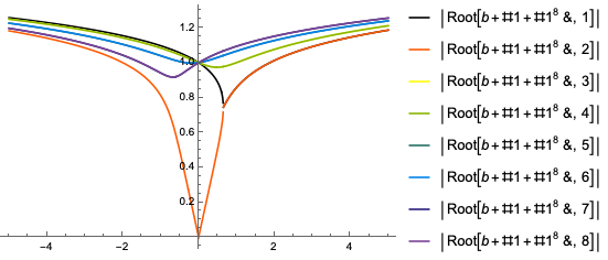
In session 16, Symbolic Mathematics, I modified some code in subsection "Root Expressions" to get a legend on the plotted output. My modified code is:
In[24]:= sol=Solve[x^8+ x+b==0,x]
Plot[Abs[x/.sol],{b,-5,5},PlotRange->All,PlotLegends->Automatic]
Here is the output of the first line of code:
Out[24]= {{x->Root[b+#1+#1^8&,1]},{x->Root[b+#1+#1^8&,2]},{x->Root[b+#1+#1^8&,3]},{x->Root[b+#1+#1^8&,4]},{x->Root[b+#1+#1^8&,5]},{x->Root[b+#1+#1^8&,6]},{x->Root[b+#1+#1^8&,7]},{x->Root[b+#1+#1^8&,8]}}
The second line of code includes my added option "PlotLegends->Automatic" but it does not result in any legends. I guess the reason has to do with the form of Out[24] which is the value assigned to sol. Please explain why "PlotLegends->Automatic" doesn't work here and what code will generate legends in the Plot. Attached as file GDorfmanPlot_26apr22.nb is a copy of the graph in which I have interactively colored the curves representing the absolute values (i.e., lengths of the complex values) of the solutions as functions of b. There are 4 rather than 8 curves. I assume this is because the solutions come in conjugate pairs.
Attachments:
|
|
|
Something like this?
Plot[Evaluate[Abs[x /. sol]], {b, -5, 5},
 PlotRange -> All,
 PlotStyle -> ColorData[3, "ColorList"],
 PlotLegends -> "Expressions"]
|
|
|
@Thomas Ray Worley please feel free to email wolfram-u@wolfram.com if you are facing issues with the notebooks. We will be happy to help you troubleshoot further. You should be able to open all the notebooks in the same way.
|
|
|
Week 1 Review notebook added to download folder.
|
|
|
Thanks Richard. That second reason should always be kept in mind.
|
|
|
Thanks Richard. It appears that f[x_] := f[x] =. .. is more efficient. Is there ever a case in which it should not be used?
|
|
|
You would probably not want to use this if the function was unlikely to be frequently called with the same argument. You would DEFINITELY NOT want to use it if you need the function to return different results when called with the same argument (e.g. if the result depended on some extermal value such as the current time or any of the Random* functions).
|
|
|
Thanks for the response and explanation, @Richard Hewens SetDelayed OR Set should serve well in defining a function. Here is an example of where using Set and SetDelayed together is helpful and might explain why it would be not advisable to try and use them together ALL the time. In the following example, when the need arises to store some constant values, immediate assignments are made. On the other hand, to store a more generic definition of the function, delayed assignment is used:
fib[0] = 0;
fib[1] = 1;
fib[n_] := fib[n] = fib[n - 1] + fib[n - 2]
The use of both Set and SetDelayed allows assignments to be made dynamically:
?fib
The Wolfram Language provides automatic recursion, coded into the delayed assignment definition of fib[n_]. Each time a new n is used, a new value for the function fib is defined and stored away. This avoids having to return all the way to the base case for every value that is used:
fib[3]

?fib

Trace[fib[4]]

Clear[fib]
|
|
|
When defining functions, when is it better to use f[x_] := f[x] =. ..instead of just f[x_] := ...? Why?
|
|
|
When using the "f[x_] := f[x]=...", this is creating a more specific function with the same name (which will be called before the original f[x_] form). This is most useful when the function will be called multiple times with the same argument, is which case the computation will only need to be done once.
|
|
|
Can someone explain this curious behavior of the Defer function:
Defer[Plus[0, 1, 2, 3, 4, 0, 1, 2, 3, 4]] results in 0 + 1 + 2 + 3 + 4 + 0 + 1 + 2 + 3 + 4, but
Defer[Times[0, 1, 2, 3, 4, 0, 1, 2, 3, 4]] results in 0 x 2 x 3 x 4 x 0  x 2 x 3 x 4
It appears that Defer somehow "knows" that any 1's can be removed from a product without affecting the result (but doesn't remove the 0s from a sum) . My first thought was that Plus and Times might have different attributes, but they were identical. Any clues to what's going on here will be appreciated.
|
|
|
Hi Richard—I'm looking into this. For the time, I can note that it's not a property of Defer, since Hold and Unevaluated (at least) do the same thing. The current thought is that it's a formatting property of Times, and formatting is a bit of an arbitrary choice that language designers have to make. I do agree that it's strange that the additive identity does not format the same way for Plus, though.
|
|
|
Bravo, Richard. You have a sharp eye. Not everyone would have noticed this nuance.
|
|
|
Based on my previous experience ( about 6 classes taken at different times), I would recommend the following.
(1) Create a notebook, say "Class3_my practice and questions". Let's call it MNB (my notebook).
(2) Open the downloaded class notebook(s), typically one or two (CNBs).
(3) The goal is to reproduce in MNB the most of activities presented in CNBs. Also, consider some variations of the offered examples, mark the difficulties and formulate the questions.
(4) In doing so, make sure to create sections in MNB ( using Alt-1 - Alt-6 shortcuts, with textual inserts using Alt-7) reflecting the corresponding sections in CNBs (so that the general structure of MNB is similar to CNB, but it may include some additional sub(-sub)sections such as "My question to the forum", or "some additional examples", or "the definition of such and such function...").
(5) Watch the pieces of the class video addressing the questionable parts (in case you do not have time to watch the whole video).
(6) As a result, you should have a few unanswered questions. Never hesitate to post them on the forum. This is good for all the participants! So, consider it a public service :)
(7) In parallel, create the notebooks Quiz1, 2, etc for solving the quiz problems. Each lecture contains (hints to) the answers to some Quiz questions. Doing it continually makes the Quiz activities less stressful (make sure not to discuss directly the Quiz questions on the forum, but you can discuss any related general issues ). Good luck.
|
|
|
This is really helpful - thank you!
|
|
|
Please post more 'stackoverflow'-like post like this in the future... it benefits a LOT.. on a very LONG run..
|
|
|
Thank you. :-) Class is going a bit rapidly. Consequently, I like to work the notebooks and exercises after class in the evening to reinforce my learnings. I am very much enjoying the classes, but there are so many new ideas and insights every day that it takes some time and practice to internalize the use and application of all the tools we have been exposed to. What is the best way to get more practice?
|
|
|
With more than 24 new functions per second, one probably has to assume a movie. Nevertheless, the study group is absolutely fascinating, and offers many new insights.
|
|
|
Responding to multiple-choice Qs does not contribute to certification. It's for self-testing. Watching the lectures and passing the quizzes do.
|
|
|
That is correct. Thanks Michael. The requirement for certificate of Program Completion for the study group is attending the live sessions and passing the online quizzes with a score of at least 60%. We will release 3 quizzes over the entire duration of this 3-week study group and you will have time till may 13th to complete all the quizzes.
|
|
|
I need to regroup for a trip that starts Monday. For that time I will switch to a cloud account and need to arrange file directories. (1) How to (up)load their files for the class? (2) How to order them based on the sessions' order number?
. The ordering turned out to be especially ticky.
Thank you
|
|
|
Hi, I can watch the lectures as a recorded video. Is there an another way to get certificate of progtam completion rather than solving multiple choices problems on live sessions?
|
|
|
Are we able to get copies of the exercises so we can work them offline to ensure we understand?
Thank you!
|
|
|
Posted exercises for days 1, 2 and 3 in the series download folder.
|
|
|
Hello, Abrita, and thank you.
M
|
|
|
Is it possible to access the NB files and quizzes for this class in the cloud?
|
|
|
Hello Michael, While the notebooks are only available in the downloadable form right now, they will soon be available as part of the new interactive course on the Wolfram U site (as cloud notebooks). We just do not have a confirmed release date for that course yet. The quizzes (with multiple choice questions) to be completed for Certificate of Program Completion will definitely be available on the cloud - same a other Daily Study Groups so far. If you are referring to the programming exercises we added to the download folder, I think we can try to share cloud published versions of the exercises by the end of the week.
|
|
|
Please help me to fix this attempt to modify the p in addition to q and r:
Range[10]/.{p___,q_,r_} -> { #^2&/@p, q r }
(motivated by the 1st example from the 'Rule-Based Programming' section of the first class NB). Also, transformation p-> 2*p leads to a strange result:
In[37]:= Range[10] /. {p___, q_, r_} -> {2 p, q r} Out[37]= {**80640**, 90}
Thanks.
M PS What is wrong with using #^2&/@p where p corresponds to 8 initial elements of the list, given that
"#^2&/@Range[8]" works as expected.
|
|
|
The following code should explain what parts of the expression Range[10] are matching p, q and r:
Range[10] /. {p___, q_,
r_} -> {{"This is p: ", p}, {"This is q: ", q}, {"This is r: ", r}}
This is the output you get:
{{"This is p: ", 1, 2, 3, 4, 5, 6, 7, 8}, {"This is q: ", 9}, {"This is r: ", 10}}
So what is essentially happening with the {#^2 & /@ p, q r} part of the expression is {#^2 & /@ 1, 2, 3, 4, 5, 6, 7, 8, q r} i.e. #^2 is mapped over the single element 1 and therefore gives the result {1, 2, 3, 4, 5, 6, 7, 8, 90} This would give the expected result:
Range[10] /. {p___, q_, r_} :> Join[#^2 & /@ {p}, {q r}]
|
|
|
Awesome! Thank you very much, Abrita.
Best.
M
|
|
|
Range[10] /. {p___, q_, r_} :> {Hold[ 2 p], q r}
shows what's happening with 2 p. It is computing 2X2X3X4X5X6X7X8 p (from the RHS of the rule) is really a fragment of an expression. It needs to be explicitly turned into a list to get the output you are looking for.
Maybe something like:
Range[10] /. {p___, q_, r_} :> Append[2 {p}, q r]
|
|
|
Abrita: "So what is essentially happening with the {#^2 & /@ p, q r} part of the expression is {#^2 & /@ 1, 2, 3, 4, 5, 6, 7, 8, q r} i.e. #^2 is mapped over the single element 1 and therefore gives the result {1, 2, 3, 4, 5, 6, 7, 8, 90}
This would give the expected result:
Range[10] /. {p__, q, r_} :> Join[#^2 & /@ {p}, {q r}]"
************************************************************************** Thanks!
This opens a window to many opportunities such as this one:
Range[10] /. {p__, q, r_} :> Flatten[{2 {p}, {q r}}]. Yet, I still have a question: what kind of object is p without {}? In other words, what is the sequence of "bare" comma-separated numbers from the WL perspective? I understand that in our case it is a "list" of arguments. But this is not a List. What is it? Maybe you have already responded by saying that this is a fragment of an expression.. But there should be also some rules (default) telling M how to treat those...
Could you please clarify? For example, what is the rule leading to 2 p = 2X2X3X4X5X6X7X8? It even seems to contradict the treatment of p in the previous example where p was reduced to its first element (as you said, the "single element 1"). Thank you.
M
|
|
|
Hi Michael, p appears to be a Sequence. I reached out to our instructor Dave Withoff for a more complete explanation, and here is the response from Dave:
"... start with an input like
In[]:= Range[10] /. {p___, q_, r_} -> p
Out[]= Sequence[1, 2, 3, 4, 5, 6, 7, 8]
to find out exactly what expression is matched to the named pattern "p" when the rule is applied. The result here shows that "p" will be replaced by Sequence[1, 2, 3, 4, 5, 6, 7, 8]. Inserting Sequence[1, 2, 3, 4, 5, 6, 7, 8] in place of p in 2 p, or equivalently, in Times[2, p], gives Times[2, Sequence[1, 2, 3, 4, 5, 6, 7, 8]]. The Sequence expression is spliced in to the enclosing expression in an early step of evaluation to get Times[2,1, 2, 3, 4, 5, 6, 7, 8], which subsequently evaluates to the observed result. The handling of Sequence expressions will be explored in one of the last sessions of the study group series."
Hope this helps.
|
|
|
Dear Arbita and Dave. Your responses are very valuable, especially by teaching how to "huck" it (look under the hood). There is a lot to digest. Thank you.
M
|
|
|
Michael—sequences can indeed be a little tricky, but they're a great tool to add to your arsenal. You can really start manipulating things at a low level once you have a grasp on them and how they work with patterns!
|
|
|
Thank you, Arben, At first sight, it indeed seems so .... insignificant :(. I am sure that it is а misleading impression. This happens with everything really basic.
|
|
|
Hi Abrita! The first chunk you posted:
Range[10] /. {p___, q_, r_} :> {Hold[ 2 p], q r}
...helped me find a solution to something related to what
Richard Hewens posted. I found a different solution but I like yours so much better. THANK YOU! :-D
|
|
|
Caesar Cipher example and Day 1 exercises have been added to the download folder.
|
|
|
Where is the link to the download folder?
|
|
|
Hi Syd, The link is included in the reminder emails you have been receiving from the Wolfram U Team. It is also shared during the session.
|
|
|
Hi Joel,
You can join the Wolfram Community and participate in any discussion thread. This particular thread is dedicated to the Daily Study Group: A Guide to Programming and Mathematics with the Wolfram Language. You can click on "Follow this Post" to receive notifications of any activity on this thread.

|
|
|
Dear Abrita.
Due to the trip, my deadline was shifted till today. I submitted the solutions to three quizzes. In the last quiz, four problems were accepted, and one was rejected. I sent a file describing my solution to the rejected problem and asked to check if it was really wrong. It was sent to Wolfram-U, with attention to you and Arben. I do not worry about the final score but would like to understand the reason for rejection. Could you please help me with this? Thank you. Michael.
|
|
|
@Michael Partensky sometimes the auto-grader is unable to handle alternative solutions. All your solutions were accepted on manual grading.
|
|
|
Thank you.
The auto-grader is an interesting creature on its own. Is it one of Wolfram's projects? If it is, please post a link. What are the grading criteria (in addition to the final result), the ideas behind it, how does it learn...? Are there wider applications, e.g., for a justice system, or for use by a Supernal being judging the Humans?
Thanks again.
Michael.
|
|
|
Do we have to post a reply to join the group?
|
|
|
Reply to this discussion
in reply to
|