Extend the analysis to turbulent flows and make an unsteady analysis of the stationary flows we considered...analyze fluid flow on Arnold's Cat Map?
frames =
VideoExtractFrames[
Video["/Users/deangladish/Downloads/water.mp4",
Appearance -> Automatic, AudioOutputDevice -> Automatic,
SoundVolume -> Automatic],
Interval[{Quantity[0.0, "Seconds"], Quantity[2.0, "Seconds"]}]];
flow = ImageDisplacements[{frames[[35]], frames[[36]] }]
pts = ImageFeatureTrack[{im1 = frames[[35]], im2 = frames[[36]]},
MaxFeatures -> 20];
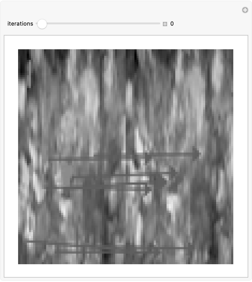
Manipulate[ArrayPlot[Nest[Compile[{{pic, _Integer, 2}},
Table[
pic[[Mod[x + y, 100, 1], Mod[x + 2 y, 100, 1]]], {x, 100}, {y,
100}]],
255 - Reverse[Map[(IntegerPart [#*255]) &,
ImageData[ColorConvert[ImageResize[
Show[ImageAssemble[{im1, im2}],
Graphics[{Green, PointSize[.02],
MapThread[
If[#2 === Missing[], {Cyan, Point[#1]},
Arrow[{#1, #2 + {ImageDimensions[im1][[1]], 0}}]] &,
pts]}]
], {100, 100}], "Grayscale"]]]], iter],
Frame -> False], {{iter, 1, "iterations"}, 0, 150, 1,
Appearance -> "Labeled"}, SaveDefinitions -> True]
@Chase Marangu and @Mohammad Ali Ghorbani just remember how insanely fast I could type and the bean bags in the building, that we sat there together. We started to study river flow velocity estimation...please tell us more we're definitely interested in video processing and animated optical fluid flows!
pts = ImageFeatureTrack[{im1 = frames[[35]],
    im2 = frames[[36]]},
   MaxFeatures -> 20];
Show[ImageAssemble[{im1, im2}],
  Graphics[{Green, PointSize[.02],
      MapThread[
        If[#2 === Missing[], {Cyan, Point[#1]},
            Arrow[{#1, #2 + {ImageDimensions[im1][[1]], 0}}]] &,
    pts]}]]
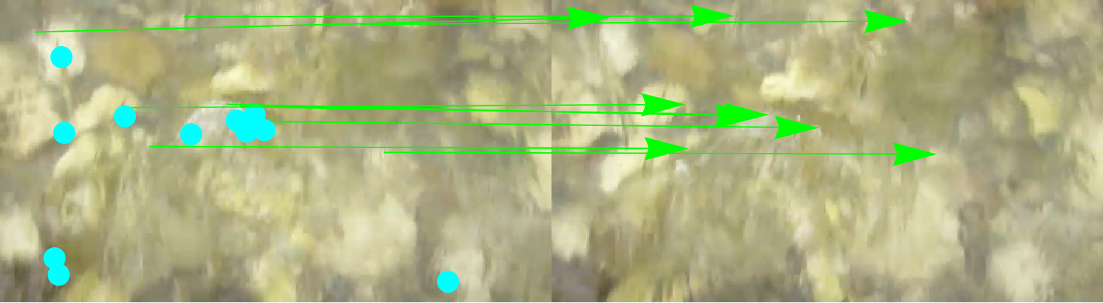
A lot of the time we try to make it too nice so just throw something together that works and work on your other assignments. The focus on the closed arrangement of pipes, it focuses how much on the study of fluid flow.
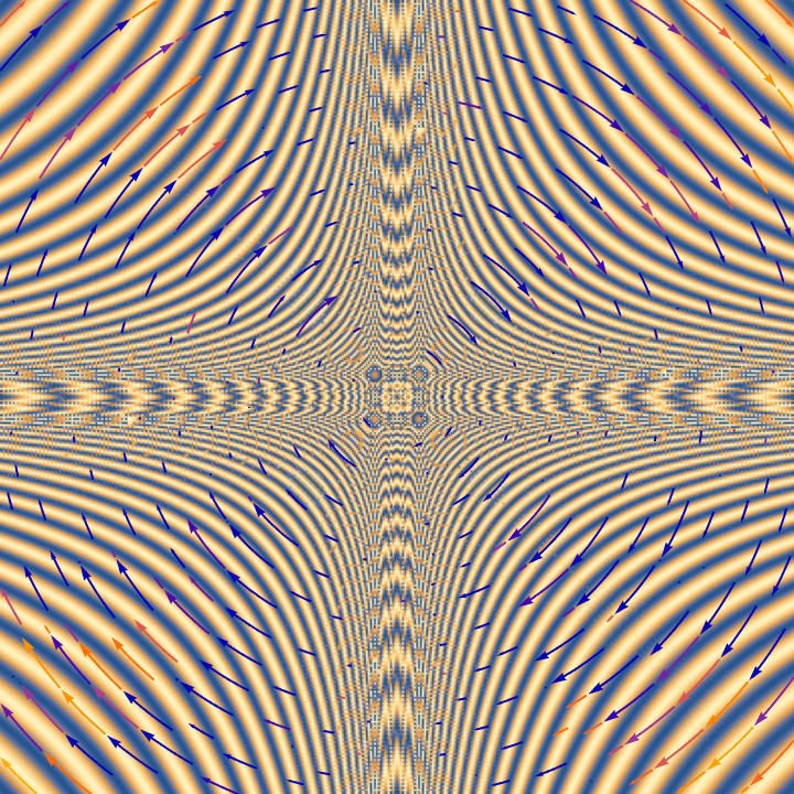
pseudoFractal[x_, y_] := Sin[12 Log[2, Abs[x y]]]^2
Show[
 DensityPlot[
  pseudoFractal[x, y],
  {x, -3, 3},
  {y, -3, 3},
  Frame -> False,
  PlotPoints -> 100,
  MaxRecursion -> 2,
  PlotRangePadding -> None,
  ColorFunction -> "M10DefaultDensityGradient"],
 StreamPlot[{
   y pseudoFractal[x, y],
   -x pseudoFractal[x, y]
   }, {x, -3, 3},
  {y, -3, 3}]]
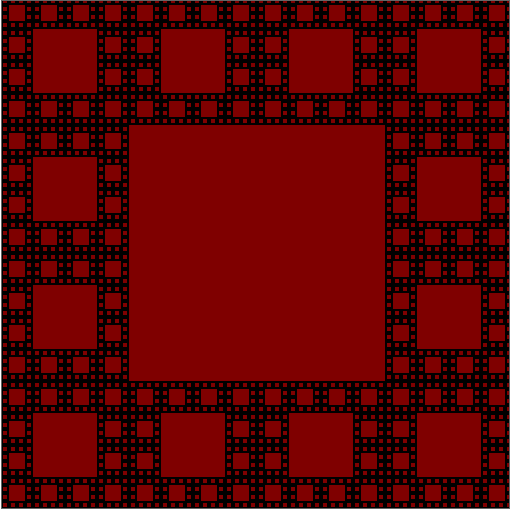
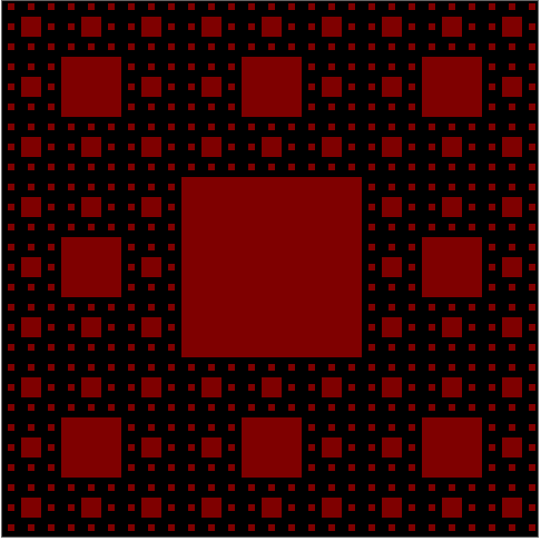
ArrayPlot[
 Nest[
  ArrayFlatten[
    {{#, #, #, #},
     {#, 0 &, 0 &, #},
     {#, 0 &, 0 &, #},
     {#, #, #, #}}] &,
  {{1}},
  4], PixelConstrained -> True]
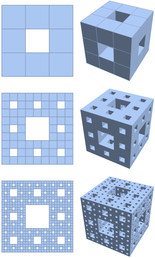
We do use the finite elements method. The Navier-Stokes equations and the cutoff of the energy conservation equation are taken into this fractal. We don't take the behavior of laminar flows and we do take into account the Navier-Stokes equations and the energy conservation equation, just not in the conventional sense. The Menger Sponge and the Sierpinski are the three-dimensional and two-dimensional fractals and it really does come down to fractals. These, are some easy patterns.
ArrayPlot[
 Nest[
  ArrayFlatten[
    {{#, #, #},
     {#, 0 &, #},
     {#, #, #}}] &,
  {{1}},
  4], PixelConstrained -> True]
I wouldn't be surprised if at some moment the laminar flow has both stationary and unsteady behavior on fractal meshes and as a result boundary conditions are crucial to this behavior, including both temperature and pressure gradients between the walls. That is even possible that it's right for the Navier-Stokes equations to be solved, that's the powerful reputation of the computational fluid dynamics..
Manipulate[
 StreamPlot[
  {Cos[x + a], Sin[y + a]},
  {x, -3, 3}, {y, -3, 3}],
 {a, -2, 2}]
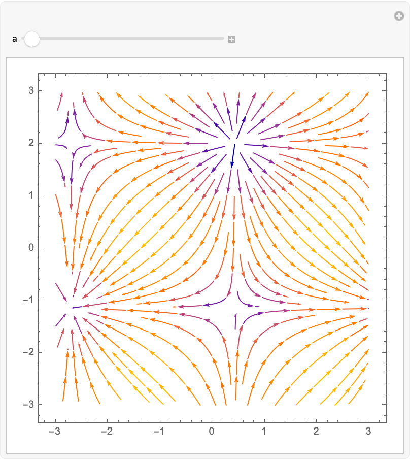
I'm dating myself by saying that.. I'm sorry. There are a countless number of computational fluid dynamics. That was an out of bounds simplified representation. All I want is to base it, for physical equations of fluid dynamics, and there's also something else..the sufficient "feel" of a fluid. Let's just leave it at the fluid-like animation, where I use this sine and cosine vector field.
GraphicsGrid[Table[MengerMesh[n, s], {n, 3}, {s, 2, 3}],
 Frame -> None]
catMengerMesh[n_, scale_] :=
  Nest[DeleteCases[
     Flatten[Table[
       If[(i == 2 && j == 2) || (j == 2 && k == 2) || (k == 2 &&
           i == 2), {},
        Cuboid[Pi*#[[1]] + {i, j, scale*k}/3] & /@ #], {i, 0, 2}, {j,
        0, 2}, {k, 0, 2}], 1], {}, Infinity] &, {Cuboid[{0, 0, 0}]},
   n];
animation =
  Animate[Show[
    ParametricPlot3D[{t, Sin[t + a], 0}, {t, 0, 2*Pi},
     PlotStyle -> {Dashing[0.01], Thickness[0.001], Blue}],
    Graphics3D[{Directive[Opacity[0.2],
       ColorData["RedBlueTones"][Sin[a]]], catMengerMesh[1, Sin[a]]}],
     PlotRange -> {{-1, Pi}, {-1, 1}, {-1, 2}}, Axes -> True,
    Boxed -> True, Lighting -> "Standard"], {a, 0, 2*Pi, Pi/15}];
There that was the gradient of pressure fluid flow in the opposite direction; the Reynolds number is used to confirm the laminar flow. Now we've got this fake pressure-driven flow. We can make the flow more laminar, it seems. We could also refine the fractal domain flow to meshes corresponding to more iterations of the fractal construction process, on the way out.
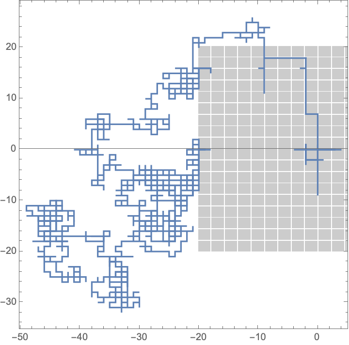
numSteps = 2000;
walk = {{0, 0}};
squares = Flatten[
   Table[
    {{i, j}, {i + 2, j + 2}},
    {i, -20, 20, 2.25},
    {j, -20, 20, 2.25}], 1];
insideSquareQ[pt_, squares_] := AnyTrue[squares,
   (pt[[1]] > #[[1, 1]] &&
      pt[[1]] < #[[2, 1]] &&
      pt[[2]] > #[[1, 2]] &&
      pt[[2]] < #[[2, 2]]) &];
randomStep[pt_] := Module[
   {step = RandomChoice[{{-1, 0},
       {1, 0},
       {0, -1},
       {0, 1}}]},
   While[insideSquareQ[pt + step, squares],
    step = RandomChoice[{{-1, 0},
       {1, 0},
       {0, -1},
       {0, 1}}]]; step];
Do[AppendTo[walk, Last[walk] + randomStep[Last[walk]]],
  {numSteps}];
ListPlot[walk, Joined -> True, AspectRatio -> 1, Frame -> True,
 Prolog -> {Opacity[0.2], Rectangle @@@ squares}]
There's no guide for animated optical fluid flows..the temperature-controlled flow operators could also be experimented with under boundary conditions. It turns out that this is just a three-dimensional extension of the Sierpinski carpet, the Menger Sponge is using a similar mesh function in a higher dimension.
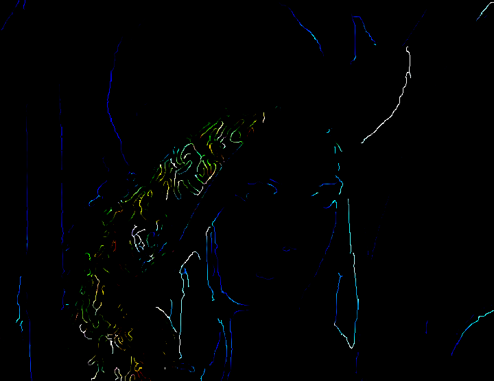
Show[ImageSubtract[EdgeDetect[#], ImageAdjust[#, {2, 2}]] &@
  ImageResize[Import["ExampleData/lena.tif"], 700]]
To keep the character of these pressure-driven flows, in a domain where a higher iteration number results in a higher Reynolds number, implying a trend as iteration order increases, a trend towards turbulence whereas on the contrary, in temperature-driven flows, a higher iteration number led to a lower Reynolds number, making a more laminar flow. Supposedly this flow has many characteristics and patterns.


