Dear Joe,
here are some ideas:
1) this is what you download:
datatimes = FinancialData["VO", "Return", "Jun. 26, 2004"];
as you say it contains the dates.
2) you only take the magnitudes for each day.
data = datatimes[[All, 2]];
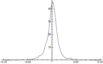
3) you can calculate a smooth kernel distribution
Plot[PDF[SmoothKernelDistribution[data], x], {x, -0.1, 0.1}, PlotRange -> All]
4) this generates the product of a random choice of 252 returns:
Product[RandomChoice[data, 252][[i]], {i, 1, 252}]
It does not help a lot because it is numerically nearly always zero - on the bright side it is probably not what you want to calculate anyway.
The mean of the returns is
Mean[data]
which evaluates to 0.000551085. The standard deviation is
StandardDeviation[data]
which is 0.0144021. The product of many numbers that come from such a narrow distribution around zero can become very small. Also
Min[Abs[data]]
is 0. Actually,
Sort[Abs[data]]
gives:
{0., 0., 0., 0., 0., 0., 0., 0., 0., 0., 0., 0., 0., 0., 0., 0., 0., 1.1102210^-16, 1.1102210^-16, 0.00010582, 0.000108319, 0.00011383, 0.000118779, 0.000120048, 0.000123977, 0.000124425, 0.000124,....}
If any of the first numbers are in your random choice you get zero.
5) Luckily, to get an average return you might not want to multiply the data but rather sum them up
Sum[RandomChoice[data, 252][[i]], {i, 1, 252}]
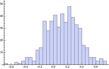
6) The histogram of that is:
Histogram[Table[Sum[RandomChoice[data, 252][[i]], {i, 1, 252}], {k, 1, 500}], 20]
7) The mean over 500 of these realisations can be obtained like so:
Mean[Table[Sum[RandomChoice[data, 252][[i]], {i, 1, 252}], {k, 1, 500}]]
I got 0.149755 when I ran it for my realisation. This seems to be more or less ok, because the average daily return was 0.000551085. Multiplying this by 252 gives 0.138873.
8) Let's see. If we run the entire thing say 100 times
Monitor[Table[Mean[Table[Sum[RandomChoice[data, 252][[i]], {i, 1, 252}], {k, 1, 500}]], {j,1, 100}], j]
we get
{0.130739, 0.1443, 0.12358, 0.127578, 0.123799, 0.127366, 0.137378, \
0.142802, 0.123663, 0.131705, 0.143079, 0.129468, 0.133854, 0.152172, \
0.14965, 0.124151, 0.148038, 0.129823, 0.124735, 0.142115, 0.13393, \
0.146552, 0.142295, 0.145668, 0.148012, 0.149947, 0.157339, 0.144625, \
0.131332, 0.152722, 0.152528, 0.132397, 0.149237, 0.133508, 0.147617, \
0.133868, 0.1329, 0.155013, 0.144509, 0.139821, 0.1457, 0.160008, \
0.140802, 0.122112, 0.139138, 0.147673, 0.136278, 0.142777, 0.117216, \
0.113688, 0.142883, 0.132171, 0.140114, 0.146726, 0.142973, 0.15172, \
0.136722, 0.141169, 0.128717, 0.1394, 0.138362, 0.145236, 0.151213, \
0.13936, 0.123638, 0.12851, 0.140283, 0.139783, 0.12457, 0.137845, \
0.13261, 0.153618, 0.126994, 0.127699, 0.137892, 0.15243, 0.151824, \
0.131615, 0.135664, 0.134355, 0.144779, 0.126877, 0.135637, 0.129136, \
0.144117, 0.139079, 0.144863, 0.13009, 0.142233, 0.127004, 0.118718, \
0.154026, 0.137453, 0.111452, 0.148349, 0.137895, 0.140912, 0.116243, \
0.134876, 0.129615}
The mean of that
Mean[%]
is 0.137787. And the variance is
Variance[%%]
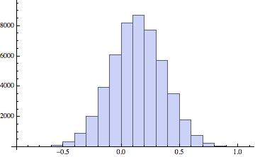
0.000106633 and the standard deviation is 0.0103263. So after altogether 500*100=50000 realisations we are quite close to the theoretical value of 0.138873. We now can calculate the histogram from point 6 for 50k realisations:
Monitor[Histogram[Table[Sum[RandomChoice[data, 252][[i]], {i, 1, 252}], {k, 1, 50000}], 20], k]
This gives the really smooth histogram
8) I suppose that to a very good approximation that is Gaussian distributed. Let's check that.
DistributionFitTest[datalist, Automatic, "TestConclusion", SignificanceLevel -> 0.05]
Results:
The null hypothesis that the data is distributed according to the
NormalDistribution[[FormalX],[FormalY]] is not rejected at the 5.
percent level based on the Cramér-von Mises test.
If we fit a Gaussian and then plot them together we get:
Show[Histogram[datalist], Plot[1000*PDF[EstimatedDistribution[datalist, NormalDistribution[\[Mu], \[Sigma]]], x], {x, -1, 1.2}, PlotStyle -> {Red, Thick}]]
This give this nice figure:
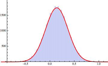
With this it becomes easy to make all sorts of nice predictions. Oh, yes, here are the parameters I got for the distribution:
EstimatedDistribution[datalist, NormalDistribution[\[Mu], \[Sigma]]]
gives: NormalDistribution[0.137692, 0.22852].
I hope that helps a bit. It is quite safe to ignore point 8. That one is just for fun.
Cheers,
Marco


