ABSTRACT (original article): Numerical tools for computation of ℘-functions, also known as Kleinian, or multiply periodic, are proposed. In this connection, computation of periods of the both first and second kinds is reconsidered. An analytical approach to constructing the Reimann surface of a plane algebraic curves of low gonalities is used. The approach is based on explicit radical solutions to quadratic, cubic, and quartic equations, which serve for hyperelliptic, trigonal, and tetragonal curves, respectively. The proposed analytical construction of the Riemann surface gives a full control over computation of the Abel image of any point on a curve. Therefore, computation of ℘-functions on given divisors can be done directly. An alternative computation with the help of the Jacobi inversion problem is used for verification. Hyperelliptic and trigonal curves are considered in detail, and illustrated by examples. CITATION (original article): Julia Bernatska, Computation of ℘-functions on plane algebraic curves, arXiv:2407.05632. https://doi.org/10.48550/arXiv.2407.05632
See second part here: Uniformization of a genus 3 trigonal curve
Introduction
This discussion illustrates Example 1 from the material published in arXiv:2407.05632
Uniformization of a genus 4 hyperelliptic curve $\mathcal{C}$, as an example, is suggested. This uniformization generalizes the Weierstrass uniformization of an elliptic curve: $(x,y) = \big( \wp(u), -\wp'(u)\big)$. In higher genera, $\wp$-functions known as multiply periodic after Baker [B2], or Kleinian after Buchstaber, Enolski, and Leykin [BEL], arise:
$\wp_{i,j}(u) = - \dfrac{\partial^2}{\partial u_i \partial u_j} \log \sigma(u),\qquad \wp_{i,j,k}(u) = - \dfrac{\partial^3}{\partial u_i \partial u_j \partial u_k} \log \sigma(u).$
Then every positive non-special divisor $D_g$ of degree $g$, equal to the genus of a curve, is expressed in terms of a particular collection of $2g$ $\wp$-functions. On one hand, these functions can be computed at $u \in \mathrm{Jac}(\mathcal{C})$ which serves as the Abel image of $D_g$. On the other hand, $\wp$-functions are expressed in terms of symmetric functions in coordinates of the support of $D_g$. And this correspondence serves as uniformization.
Indeed, the Abel image $\mathcal{A}(P)$ of any point of a curve $P$ can be computed directly, and so the image $\mathcal{A}(D)$ of a divisor $D$ of any collection of points:
$D = \sum_{j=1}^N P_j$ $\quad\Rightarrow\quad$ $\mathcal{A} (D) = \sum_{j=1}^N \mathcal{A} (P_j$).
On the other hand, the Jacobi inversion problem provides a one-to-one correspondence $\mathrm{Jac}(\mathcal{C}) \leftrightarrow \mathcal{C}^g$ between the Jacobian variety $\mathrm{Jac}(\mathcal{C})$ of the curve, and its $g$-th symmetric power $\mathcal{C}^g$. Thus, every positive non special divisor $D_g$ of degree $g$ is completely determined by a pair of entire rational functions on the curve:
$\mathcal{R}_{2g}(x;u) = x^g - \sum_{i=1}^g x^{g-i} \wp_{1,2i-1}(u),$
$\mathcal{R}_{2g+1}(x,y;u) = 2y + \sum_{i=1}^g x^{g-i} \wp_{1,1,2i-1}(u).$
That is, if $u=\mathcal{A}(D_g)$, then the system: $\mathcal{R}_{2g}(x;u)=0$, $\mathcal{R}_{2g+1}(x,y;u)=0\ $ defines $D_g$ uniquely. Coefficients of the two entire rational functions (or simply polynomials in $x$ and $y$) are expressed in terms of a particular collection of $2g$ $\wp$-functions:
$\{\wp_{1,1}, \wp_{1,3}, \dots, \wp_{1,2g-1}, \wp_{1,1,1}, \wp_{1,1,3}, \dots, \wp_{1,1,2g-1}\}$ .
Below an example of genus $4$ hyperelliptic curve is explained in detail.
Curve
We work with canonical forms of hyperelliptic curves, given by $(n,s)$-curves, since $\sigma$-function is defined on this type of curves. In genus $4$, $(2,9)$-curve serves as canonical. It is defined by the equation
$$0=f(x,y)=-y^2+\mathcal{P}(x),$$
$$\mathcal{P}(x)=x^9+\lambda_2 x^8 + \lambda_4 x^7+\lambda_6 x^6 + \lambda_8 x^5+\lambda_{10}x^4 + \lambda_{12} x^3 +\lambda_{14} x^2 + \lambda_{16} x + \lambda_{18}.$$
Parameters $\lambda$ of the curve are labeled by their Sato weights: $\mathrm{wgt}\, \lambda_k=k$, and $\mathrm{wgt}\, x=2$, $\mathrm{wgt}\, y=9$.
We fix the curve by its branch points $\{(e_i,0)\}_{i=1}^9$, which are
$$ e_1 = -18 - 2 \imath,\quad e_2= -16 + 5 \imath,\quad e_3 = -11 + 3 \imath,\quad e_4 = -10 - \imath, \quad e_5 = -4 + 2 \imath, $$
$$ e_6 = -3 + 3 \imath,\quad e_7 = 3 + 3 \imath,\quad e_8 = 7 - 2 \imath,\quad e_9 = 13 - \imath. $$
Values $\{e_i\}_{i=1}^9$ are sorted ascendingly first by the real part, then the imaginary part.
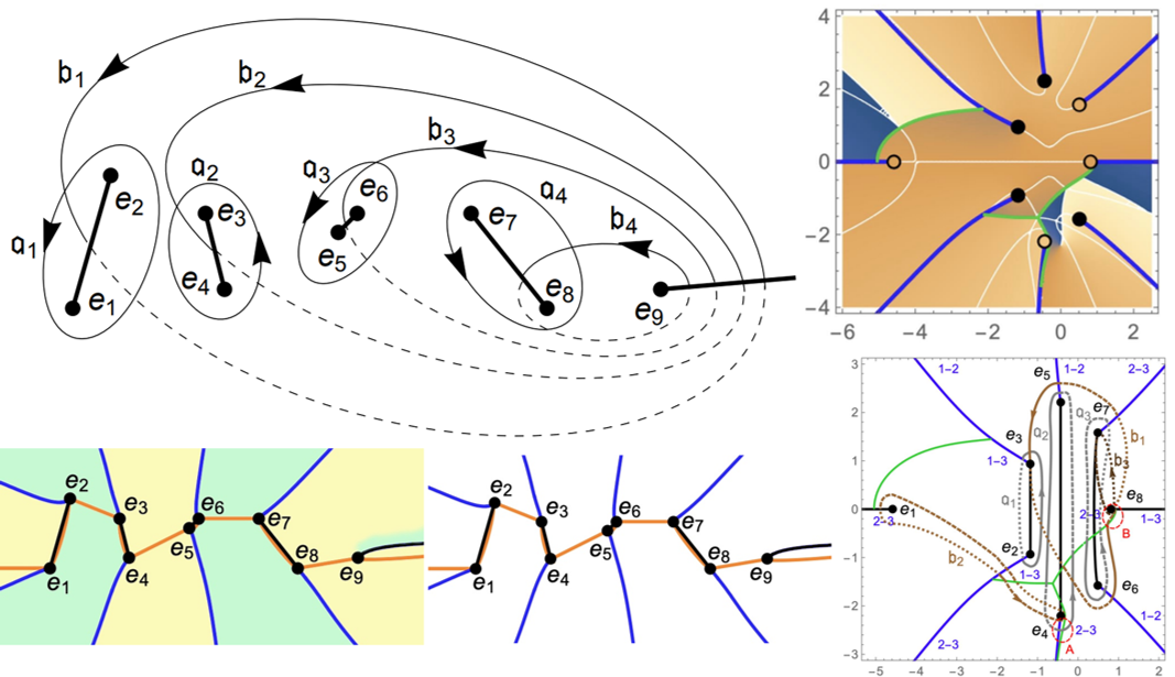
Canonical homology basis
Cuts are made between points $e_{2k−1}$ and $e_{2k}$ with $k$ from $1$ to $g=4$, and from $e_9$ to infinity ∞. An $\mathfrak{a}_k$-cycle encircles the cut $(e_{2k−1},e_{2k}$) counter-clockwise, and a $\mathfrak{b}_k$-cycle enters into the cut ( $e_{2k−1},e_{2k}$) and emerges from the cut $(e_9, ∞)$, see the figure 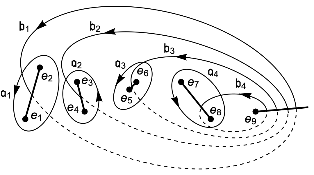
Cohomologies
First kind differentials (not normalized) have the standard form $$ \mathrm{d} u = \begin{pmatrix} \mathrm{d} u_1 \\ \mathrm{d} u_3 \\ \mathrm{d} u_5 \\ \mathrm{d} u_7 \end{pmatrix} = \begin{pmatrix} x^3 \\ x^2 \\ x \\1 \end{pmatrix} \frac{\mathrm{d} x}{-2y}.$$ Second kind differentials associated with the standard first kind differentials are $$ \mathrm{d} r = \begin{pmatrix} \mathrm{d} r_1 \\ \mathrm{d} r_3 \\ \mathrm{d} r_5 \\ \mathrm{d} r_7 \end{pmatrix} = \begin{pmatrix} x^4 \\ 3x^5 + 2 \lambda_2 x^4 + \lambda_4 x^3 \\ 5x^6 + 4 \lambda_2 x^5 + 3 \lambda_4 x^4 + 2 \lambda_6 x^3 + \lambda_8 x^2 \\ 7 x^7 + 6 \lambda_2 x^6 + 5 \lambda_4 x^5 + 4 \lambda_6 x^4 + 3 \lambda_8 x^3 + 2 \lambda_{10} x^2 + \lambda_{12} x \end{pmatrix} \frac{\mathrm{d} x}{-2y}.$$
Differentials are labeled according to their Sato weights: $\text{wgt}\, u_{k} = -k$, $\text{wgt}\, r_{k} = k$.
Note, that $y$ acquires two values: $y_s=s \sqrt{\mathcal{P}(x)}$, where $s=\pm 1$, depending on a sheet of the Riemann surface. Below an explanation how to choose the sign $s$ is given. The square root function is defined as follows $$\sqrt{\mathcal{P}(x)} = \left\{ \begin{array}{ll} \sqrt{|\mathcal{P}(x)|}\, \mathrm{e}^{(\imath/2)\, \mathrm{arg}\,\mathcal{P}(x)} & \text{if } \mathrm{arg}\,\mathcal{P}(x) \geqslant 0, \\ \sqrt{|\mathcal{P}(x)|}\, \mathrm{e}^{(\imath/2)\, \mathrm{arg}\,\mathcal{P}(x)+\imath \pi} & \text{if } \mathrm{arg}\,\mathcal{P}(x) < 0, \end{array} \right.$$ where $\mathrm{arg}$ has the range ( $-\pi$, $\pi$]. With such a definition the range of $\mathrm{arg}\sqrt{\mathcal{P}(x)}$ is ( $0$, $\pi$]. And so $y_s$ have discontinuity over the contour $\Gamma=\{x \mid \mathrm{arg}\, \mathcal{P}(x) = 0\}$. At the same time, $y_+$ serves as the analytic continuation of $y_−$ on the other side of the contour, and vice versa. Therefore, by defining the square root function as above we fix the contour $\Gamma$ where two sheets connect. This contour is important, and its plot is required in order to construct the Riemann surface correctly.
Riemann surface
A hyperelliptic curve has two sheets, which we call Sheet 1, and Sheet 2. The sheets join at branch points. The corresponding Riemann surface is obtained by making $g+1=5$ cuts along which the two sheets are connected. Further computations require the knowledge how the sign $s$ of $y_s$ changes on each sheet. For this purpose, we draw a continuous path $\gamma$ from $-\infty$ to $\infty$ through all branch points. The figure below shows this path on the $x$-plane, in the case of the hyperelliptic curve in question. The path $\gamma$ is marked by orange. 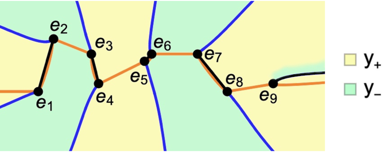 The figure also shows the contour $\Gamma$ in blue, which is a collection of segments $\Gamma_i$, each starts at $e_i$ and goes to infinity.
The path $\gamma$ goes through all $e_i$ according to the order. It is polygonal, constructed from straight line segments [ $e_i$, $e_{i+1}$], $i = 1, . . . , 8$. The segment ( $−∞$,$e_1$] is added at the beginning, and [ $e_9$,$∞$) is added at the end. It is convenient to choose the last segment coinciding with $\Gamma_9$. We assume, that $\gamma$ goes below points $\{e_i\}$, and so in the counter-clockwise direction near each $e_i$. A curved orange line near a cut shows which side of the cut is chosen.
On the figure, the whole $x$-plane is marked by two colors: yellow and green, which show the areas where $y_+$ and $y_-$, correspondingly, are located on Sheet 1. Along $\Gamma_9$, as well as every cut, Sheet 1 is connected to Sheet 2. The green area above $\Gamma_9$ indicates, that once a path crosses this segment, it enters the other sheet. The same is true for every cut: if a path enters a cut, then $y_s$ preserves the sign $s$ and the other sheet is reached. The continuous path $\gamma$ is located on one sheet, and determines the sequence of signs $s_{i,i+1}$ on its segments $[e_i,e_{i+1}]$. From the figure we see this sequence:
$\begin{array}{lcccccccccc}&\{s_{0,1},& s_{1,2},& s_{2,3},& s_{3,4},& s_{4,5},& s_{5,6},& s_{6,7}, & s_{7,8},& s_{8,9},& s_{9,0}\} =\\ \text{Sheet 1:}& \{+1, & -1, & -1, & -1, & +1, & -1,& -1,& -1, &+1, &+1\}. \end{array} $
Sheet 2 has the opposite signs of $y_s$.
Abel's map
The Abel image of a point $P \in \mathcal{C}$ is defined with respect to the not normalized differentials: $$ \mathcal{A}(P) = \int_{\infty}^P \mathrm{d} u.$$ The base point on the canonical curve, which is the $(2,9)$-curve in this case, is located at infinity, which is a branch point, and a Weierstrass point. A path from $\infty$ to $P$ starts at $-\infty$ on the real axis of $x$, and goes on the sheet where $P$ is located.
First kind integrals
Now, we compute first kind integrals between branch points along the continuous path $\gamma$: $$ \mathcal{A}_{0,1}^{[+]} = \int_{-\infty}^{e_1}\mathrm{d}u^{[+]}, \quad \mathcal{A}_{1,2}^{[-]} = \int_{e_1}^{e_2}\mathrm{d}u^{[-]},\quad \mathcal{A}_{2,3}^{[-]} = \int_{e_2}^{e_3}\mathrm{d}u^{[-]},\quad \mathcal{A}_{3,4}^{[-]} = \int_{e_3}^{e_4}\mathrm{d}u^{[-]},$$
$$ \mathcal{A}_{4,5}^{[+]} = \int_{e_4}^{e_5}\mathrm{d}u^{[+]},\quad \mathcal{A}_{5,6}^{[-]} = \int_{e_5}^{e_6}\mathrm{d}u^{[-]},\quad \mathcal{A}_{6,7}^{[-]} = \int_{e_6}^{e_7}\mathrm{d}u^{[-]},$$
$$ \mathcal{A}_{7,8}^{[-]} = \int_{e_7}^{e_8}\mathrm{d}u^{[-]},\quad \mathcal{A}_{8,9}^{[+]} = \int_{e_8}^{e_9}\mathrm{d}u^{[+]},\quad \mathcal{A}^{[+]}_{9,0} = \int^{\infty}_{e_9}\mathrm{d}u^{[+]}.$$
Here the sign $s_{i,j}$ in $\mathrm{d}u^{[s_{i,j}]}$ is chosen according to the sequence on Sheet 1. It is sufficient to compute integrals only on one sheet.
We use NIntegrate for integration from $e_i$ to $e_j$, which are given by complex numbers. This integration is performed along a line segment between $e_i$ and $e_j$. We use a line segment [ $e_i$,$e_j$] if it does not intersect $\Gamma_i$ or $\Gamma_j$, or any other segment of $\Gamma$. It could happen that a segment $\Gamma_i$ is curled around $e_i$, and a line segment to $e_j$ intersects $\Gamma_i$. In this case, a polygonal path from $e_i$ to $e_j$ should be chosen in such a way that any intersection with $\Gamma$ is avoided.
When all $\mathcal{A}_{i,j}^{[s_{i,j}]}$ along $\gamma$ are computed, we do verification. Due to the involution of a hyperelliptic curve, the following relations hold $$\mathcal{A}_{1,2}^{[-]} + \mathcal{A}_{3,4}^{[-]} + \mathcal{A}_{5,6}^{[-]}+\mathcal{A}_{7,8}^{[-]} + \mathcal{A}_{9,0}^{[+]} = 0,$$
$$ \mathcal{A}_{0,1}^{[+]} + \mathcal{A}_{2,3}^{[-]} + \mathcal{A}_{4,5}^{[+]} + \mathcal{A}_{6,7}^{[-]} + \mathcal{A}_{8,9}^{[+]} = 0.$$
If the computed $\mathcal{A}_{i,j}^{[s_{i,j}]}$ do not comply these relations, it means that something went wrong. It could be a wrong choice of a sign on an interval. Or incorrect values of some integrals due to intersection with $\Gamma$. Every time when a path crosses $\Gamma$, $y_s$ changes the sign.
First kind periods
When all integrals along $\Gamma$ are computed correctly, we calculate first kind periods according to the picture of canonical homology cycles. Actually, $\mathfrak{a}$-periods form the matrix
$\omega = 2(\mathcal{A}_{1,2}^{[-]}$, $\mathcal{A}_{3,4}^{[-]},$ $\mathcal{A}_{5,6}^{[-]},$ $\mathcal{A}_{7,8}^{[-]})$,
where $\mathcal{A}_{2k-1,2k}^{[-]}$ is a column. $\mathfrak{b}$-Periods form the matrix
$\omega' = -2 (\mathcal{A}_{2,3}^{[-]}+\mathcal{A}_{4,5}^{[+]} + \mathcal{A}_{6,7}^{[-]}+\mathcal{A}_{8,9}^{[+]}$, $\mathcal{A}_{4,5}^{[+]} + \mathcal{A}_{6,7}^{[-]}+\mathcal{A}_{8,9}^{[+]},$ $\mathcal{A}_{6,7}^{[-]}+\mathcal{A}_{8,9}^{[+]},$ $\mathcal{A}_{8,9}^{[+]})$.
The Jacobian variety is obtained from the lattice generated by columns of $\omega$ and $\omega'$, that is $\mathrm{Jac}(\mathcal{C})=\mathbb{C}^g/\{\omega,\omega'\}$.
The Riemann period matrix is obtain by normalization: $$\tau = \omega^{-1} \omega'.$$ This matrix is symmetric, with a positive imaginary part. We do verification.
Second kind integrals and periods
We compute second kind integrals along the same path $\gamma$, starting at $e_1$, ending at $e_9$: $$ \mathcal{B}_{1,2}^{[-]} = \int_{e_1}^{e_2}\mathrm{d}r^{[-]},\quad \mathcal{B}_{2,3}^{[-]} = \int_{e_2}^{e_3}\mathrm{d}r^{[-]},\quad \mathcal{B}_{3,4}^{[-]} = \int_{e_3}^{e_4}\mathrm{d}r^{[-]},$$
$$ \mathcal{B}_{4,5}^{[+]} = \int_{e_4}^{e_5}\mathrm{d}r^{[+]},\quad \mathcal{B}_{5,6}^{[-]} = \int_{e_5}^{e_6}\mathrm{d}r^{[-]},\quad \mathcal{B}_{6,7}^{[-]} = \int_{e_6}^{e_7}\mathrm{d}r^{[-]}, $$
$$ \mathcal{B}_{7,8}^{[-]} = \int_{e_7}^{e_8}\mathrm{d}r^{[-]},\quad \mathcal{B}_{8,9}^{[+]} = \int_{e_8}^{e_9}\mathrm{d}r^{[+]}.$$
Second kind periods are obtained by formulas similar to the first kind periods:
$\eta = 2(\mathcal{B}_{1,2}^{[-]}$, $\mathcal{B}_{3,4}^{[-]},$ $\mathcal{B}_{5,6}^{[-]},$ $\mathcal{B}_{7,8}^{[-]})$,
$\eta' = -2 (\mathcal{B}_{2,3}^{[-]}+\mathcal{B}_{4,5}^{[+]} + \mathcal{B}_{6,7}^{[-]}+\mathcal{B}_{8,9}^{[+]}$, $\mathcal{B}_{4,5}^{[+]} + \mathcal{B}_{6,7}^{[-]}+\mathcal{B}_{8,9}^{[+]},$ $\mathcal{B}_{6,7}^{[-]}+\mathcal{B}_{8,9}^{[+]},$ $\mathcal{B}_{8,9}^{[+]})$.
In the definition of $\sigma$-function a symmetric matrix $\varkappa$ is required: $$\varkappa = \eta \omega^{-1}.$$ We compute this matrix and verify the symmetric property.
Legendre relations
Period matrices $\omega$, $\omega'$, $\eta$, $\eta'$ form a $2g \times 2g$ period matrix $$\Omega = \begin{pmatrix} \omega & \omega' \\ \eta & \eta' \end{pmatrix},$$ which satisfies the Legendre relations, which have the matrix form $$\Omega^t J \Omega = 2 \pi \imath J,\qquad J = \begin{pmatrix} 0& -1_g \\ 1_g& 0\end{pmatrix},$$ where $1_g$ denotes the identity matrix of size $g$. In more detail, we obtain the equalities $$\eta^t \omega - \omega^t \eta = 0,$$ $$\eta'^t \omega' - \omega'^t \eta' = 0,$$ $$\eta^t \omega' - \omega^t \eta' = - 2 \pi \imath.$$ The first equality implies that $\eta \omega^{-1} = \varkappa$ is a symmetric matrix. Transposition of the matrix Legendre relations gives the equalities $$\omega' \omega^t - \omega \omega'^t = 0,$$ $$\eta' \eta^t - \eta \eta'^t = 0,$$ $$\omega' \eta^t - \omega \eta'^t = - 2 \pi \imath.$$ The first one implies that $\omega^{-1} \omega' = \tau$ is a symmetric matrix.
Verification of the Legendre relations completes computation of first and second kind periods on the curve.
Computation of $\wp$-functions
As indicated in Introduction, $\wp$-functions are defined through $\sigma$-function, which is the unique entire function invariant under integer shifts on the period lattice. Following [B1,B2], $\sigma$-function is defined as a modification of the Riemann theta function $\theta$: $$\sigma(u) = C \exp\big({-}\tfrac{1}{2} u^t \varkappa u\big)\, \theta[K](\omega^{-1} u; \omega^{-1} \omega').$$ The characteristic $[K]$ of the vector of Riemann constants on the genus $4$ hyperelliptic curve with the canonical homology basis defined above is $$[K] = \begin{pmatrix} 1 & 1 & 1 & 1 \\ 0 & 1 & 0 & 1 \end{pmatrix}.$$ Then $\wp$-functions are computed by the formulas $$\wp_{i,j}(u) = \varkappa_{i,j} - \dfrac{\partial^2}{\partial u_i \partial u_j} \log \theta[K](\omega^{-1} u; \omega^{-1} \omega'),$$ $$\wp_{i,j,k}(u) = - \dfrac{\partial^3}{\partial u_i \partial u_j \partial u_k} \log \theta[K](\omega^{-1} u; \omega^{-1} \omega').$$ The Riemann theta function is approximated by a partial sum of the Fourier series (we take $n_i$ up to 5) $$\theta(v;\tau) = \sum_{n\in \mathbb{Z}^g} \exp \big(\imath \pi n^t \tau n + 2 \imath\pi n^t v\big),$$ and a theta function with characteristic $[\varepsilon] = (\varepsilon',\varepsilon)^t$ is $$\theta [\varepsilon] (v; \tau) = \exp \big( \imath \pi (\tfrac{1}{2} \varepsilon'^t) \tau (\tfrac{1}{2} \varepsilon') + 2\imath \pi (v + \tfrac{1}{2} \varepsilon )^t (\tfrac{1}{2} \varepsilon')\big) \theta (v+ \tfrac{1}{2} \varepsilon +\tau (\tfrac{1}{2} \varepsilon'); \tau ). $$
$\wp$-Functions can be computed on non-special divisors. On a hyperelliptic curve of genus $g$ such a divisor has degree $g$ or greater, and contains no pairs of points in involution. On special divisors $\sigma$-function vanishes, and so $\wp$-functions have singularities.
The argument $u$ of $\wp$-functions is a point on the Jacobian variety $\mathrm{Jac}(\mathcal{C})$ defined with respect to not normalized periods. Thus, $u$ can be obtained as the Abel image of a non-special divisor $D$. A divisor is composed of points, and we compute the Abel image point by point.
Example 1a
Let a divisor $D$ be composed of $4$ points: $$P_1 = \big({-}9 + \imath, \sqrt{\mathcal{P}(-9 + \imath)} \big) \approx (-9 + \imath, -2174.22 + 7969.98 \imath ) ,$$ $$ P_2 = \big({-}4 - 3 \imath, \sqrt{\mathcal{P}(-4 - 3 \imath)}\big) \approx (-4 - 3 \imath, -22311.3 + 11311.5 \imath) , $$ $$ P_3 = \big(1 + 2 \imath, \sqrt{\mathcal{P}(1 + 2 \imath)}\big) \approx (1 + 2 \imath, 2721.89 + 13483.7 \imath),$$ $$ P_4 = \big(6 + 4 \imath, \sqrt{\mathcal{P}(6 + 4 \imath)}\big) \approx (6 + 4 \imath, -44563.1 + 19764.5 \imath).$$ On the figure $x$-coordinates of the points are marked in red. 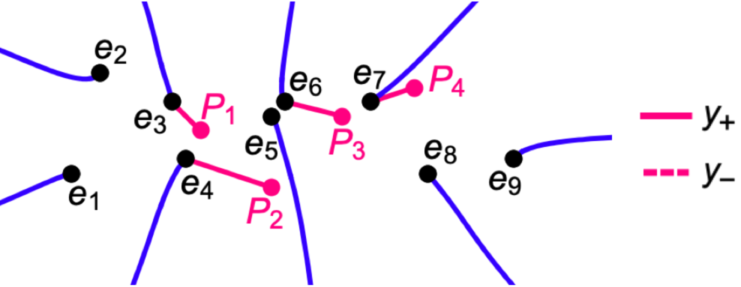
All $y$-coordinates are values of $y_+$. As we see from the previous figure, points $P_1$, $P_2$, and $P_4$ are located on Sheet 1, and $P_3$ on Sheet 2. Then, we calculate the Abel images. Choosing a path to $P$, we use the continuous path $\gamma$ to a point $e_i$ which is close to $P$, such that on the segment [ $e_i$,$P$] the sign of $y_s$ does not change. These segments are shown on the figure in red. Actually,
$$ \mathcal{A}(P_1) = \mathcal{A}_{0,1}^{[+]} + \mathcal{A}_{1,2}^{[-]} + \mathcal{A}_{2,3}^{[-]} + \int_{e_3}^{P_1} \mathrm{d} u^{[+]}. $$
$$ \mathcal{A}(P_2) = \mathcal{A}_{0,1}^{[+]} + \mathcal{A}_{1,2}^{[-]} + \mathcal{A}_{2,3}^{[-]} + \mathcal{A}_{3,4}^{[-]} + \int_{e_4}^{P_2} \mathrm{d} u^{[+]}. $$
$$ \mathcal{A}(P_3) = - \big(\mathcal{A}_{0,1}^{[+]} + \mathcal{A}_{1,2}^{[-]} + \mathcal{A}_{2,3}^{[-]} + \mathcal{A}_{3,4}^{[-]} + \mathcal{A}_{4,5}^{[+]} + \mathcal{A}_{5,6}^{[-]} + \int_{e_6}^{P_3} \mathrm{d} u^{[-]} \big), $$
$$ \mathcal{A}(P_4) = \mathcal{A}_{0,1}^{[+]} + \mathcal{A}_{1,2}^{[-]} + \mathcal{A}_{2,3}^{[-]} + \mathcal{A}_{3,4}^{[-]} + \mathcal{A}_{4,5}^{[+]} + \mathcal{A}_{5,6}^{[-]} + \mathcal{A}_{6,7}^{[-]} + \int_{e_7}^{P_4} \mathrm{d} u^{[+]}. $$
Paths to $P_1$, $P_2$, and $P_4$ go on Sheet 1, and to $P_3$ on Sheet 2. The Abel images are computed directly by integration with the help of NIntegrate. Then the Abel image of $D$ is obtained
$$ \mathcal{A}(D) = \mathcal{A}(P_1) + \mathcal{A}(P_2) + \mathcal{A}(P_3) + \mathcal{A}(P_4).$$
The divisor $D$ is uniquely represented by the corresponding values of eight $\wp$-functions:
$$\wp_{1,1}(\mathcal{A}(D)), \ \wp_{1,3}(\mathcal{A}(D)), \ \wp_{1,5}(\mathcal{A}(D)), \ \wp_{1,7}(\mathcal{A}(D)),$$
$\qquad\qquad\qquad\qquad\qquad\quad \wp_{ 1,1,1} ( \mathcal{A} (D) ), \ \wp_{ 1,1,3} ( \mathcal{A} (D) ), \ \wp_{ 1,1,5} ( \mathcal{A} (D) ), \ \wp_{ 1,1,7} ( \mathcal{A} (D) ). $
These values serve as coefficients of the entire rational (polynomial) functions $\mathcal{R}_8$, $\mathcal{R}_9$, which give a solution of the Jacobi inversion problem for $u= \mathcal{A}(D)$. Namely,
$$\mathcal{R}_8(x;u) = x^4 - x^3 \wp_{1,1}(u) - x^2 \wp_{1,3}(u) - x\, \wp_{1,5}(u) - \wp_{1,7}(u), $$
$$\mathcal{R}_9(x,y;u) = 2y + x^3 \wp_{1,1,1}(u) + x^2 \wp_{1,1,3}(u) + x\, \wp_{1,1,5}(u) + \wp_{1,1,7}(u). $$
We compare these coefficients with the ones obtained from coordinates of the points $P_1$, $P_2$, $P_3$, $P_4$. Namely, $$\mathcal{R}_8(x) = \frac{\small \begin{vmatrix} 1 & x & x^2 & x^3 & x^4 \\ 1 & x_1 & x_1^2 & x_1^3 & x_1^4\\ 1 & x_2 & x_2^2 & x_2^3 & x_2^4 \\ 1 & x_3 & x_3^2 & x_3^3 & x_3^4\\ 1 & x_4 & x_4^2 & x_4^3 & x_4^4 \end{vmatrix}}{\small \begin{vmatrix} 1 & x_1 & x_1^2 & x_1^3 \\ 1 & x_2 & x_2^2 & x_2^3 \\ 1 & x_3 & x_3^2 & x_3^3 \\ 1 & x_4 & x_4^2 & x_4^3 \end{vmatrix}},\qquad \mathcal{R}_9(x) = \frac{\small \begin{vmatrix} 1 & x & x^2 & x^3 & y \\ 1 & x_1 & x_1^2 & x_1^3 & y_1\\ 1 & x_2 & x_2^2 & x_2^3 & y_2 \\ 1 & x_3 & x_3^2 & x_3^3 &y_3 \\ 1 & x_4 & x_4^2 & x_4^3 & y_4 \end{vmatrix}}{\dfrac{1}{2} \small \begin{vmatrix} 1 & x_1 & x_1^2 & x_1^3 \\ 1 & x_2 & x_2^2 & x_2^3 \\ 1 & x_3 & x_3^2 & x_3^3 \\ 1 & x_4 & x_4^2 & x_4^3 \end{vmatrix}},$$ where $(x_i,y_i)$ are coordinates of $P_i$.
Example 1b
We slightly modify $D$ by moving $P_3$ from Sheet 2 to Sheet 1, that is
$$ P_3 = \big(1 + 2 \imath, - \sqrt{\mathcal{P}(1 + 2 \imath)} \big) \approx (1 + 2 \imath, -2721.89 - 13483.7 \imath).$$ In this case, the path to $P_3$ goes on Sheet 1: $$ \mathcal{A}(P_3) = \mathcal{A}_{0,1}^{[+]} + \mathcal{A}_{1,2}^{[-]} + \mathcal{A}_{2,3}^{[-]} + \mathcal{A}_{3,4}^{[-]} + \mathcal{A}_{4,5}^{[+]} + \mathcal{A}_{5,6}^{[-]} + \int_{e_6}^{P_3} \mathrm{d} u^{[-]}. $$ 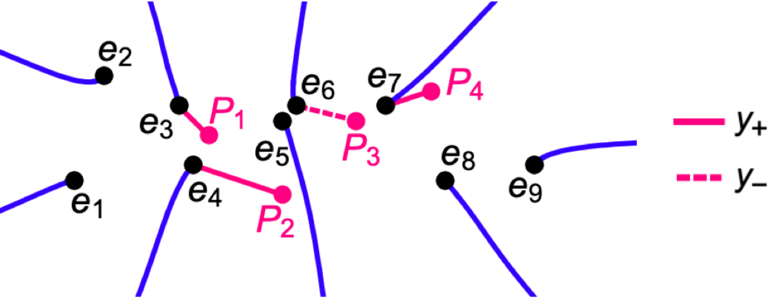
Values of $\wp_{1,1,1}(\mathcal{A}(D))$, $\wp_{1,1,3}(\mathcal{A}(D))$, $\wp_{1,1,5}(\mathcal{A}(D))$, $\wp_{1,1,7}(\mathcal{A}(D))$ change, and so the function $\mathcal{R}_9$. The new values of coefficients coincide with the ones obtained from coordinates of the points.
References
[B1] Baker H.F., Abelian functions: Abel's theorem and the allied theory of theta functions, Cambridge, University press, Cambridge, 1897.
[B2] Baker H.F., Multiply periodic functions, Cambridge Univ. Press, Cambridge, 1907.
[BEL] Buchstaber V. M., Enolskii V. Z., and Leykin D. V., Hyperelliptic Kleinian Functions and Applications, preprint ESI 380 (1996), Vienna
 Attachments:


