Click here for final result of 13 years of crime in Chicago compressed into a 1 minute animation
In a previous post I showed how to map crime data for the month of July for the City of St. Louis. In this post, I will show how to map and animate similar crime statistics for a larger city over a time span of 13 years. The city of Chicago keeps an excellent public record of all crimes committed within its boundaries. Its data access portal is fully searchable online and allows for easy download. This data access portal compares very favorably to the St. Louis crime statistics data portal which is much more dated: Download of statistics by month only, data only available for one year back, and data in a geolocation format that uses a somewhat obscure state plane coordinate system instead of simple latitude/longitude notation. It would be good if the City of St. Louis adopted the approach taken by the City of Chicago.
The first step in creating this crime animation was to download the full data set. I opted for the CSV format option, which yielded a 1.4GB data file containing all the necessary data (about 5,500,000 crimes). This imports the raw data and selects the rows containing valid dates, locations and crime types (total computation time about 288 seconds):
csv = Import["C:\\Users\\arnoudb.WRI\\Downloads\\Crimes_-_2001_to_present.csv"];
csv=Select[csv[[2;;-1,{3,6,-3,-2}]],And[#[[3]]!="",#[[4]]!=""]&];
To speed up processing of parsing of date strings into date objects, I wrote a small utility function:
dateParse[date_]:=Module[{mon,day,yr,hr,min,sec,ampm},
  {mon,day,yr,hr,min,sec,ampm}=StringSplit[date,{"/"," ",":"}];
  {mon,day,yr,hr,min,sec}=ToExpression/@{mon,day,yr,hr,min,sec};
  DateObject[{yr,mon,day,hr+12Boole[ampm==="PM"],min,sec}]
]
This maps the raw csv data into a usable data set for geographical mapping (about 1680 seconds):
data = Map[{dateParse[#[[1]]], #[[2]], GeoPosition[{#[[3]], #[[4]]}]} &, csv];
data = Reverse[data];
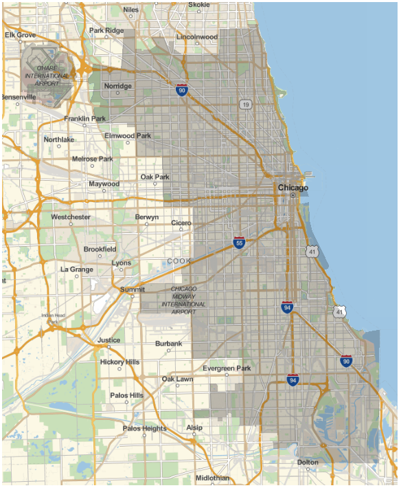
Next, we create a base geographical map for Chicago on top of which we will plot the crime data:
baseMap=GeoGraphics[{{Opacity[0.5], Polygon[Entity["City", {"Chicago", "Illinois", "UnitedStates"}]]}},
  GeoRange -> Entity["City", {"Chicago", "Illinois", "UnitedStates"}], ImageSize -> Large]

Then, we create a mapping function to map one frame of the animation. Here, index refers to the animation frame index and start and end refer to the start and end point of the data being mapped. Data points nearest to end (the most recent ones) are colored with red, fading to black for the
map[index_, start_, end_] := Export[
  StringJoin["c:\\users\\arnoudb.wri\\chicago\\frames\\crime-", IntegerString[index, 10, 4], ".png"],
  Overlay[{baseMap,
    GeoGraphics[MapIndexed[{RGBColor[N[1.0-First[#2]/(end-start)],0,0], AbsolutePointSize[4], Opacity[0.1],Point[Last[#1]]}&,data[[start ;; end]]],
    GeoRange -> Entity["City", {"Chicago", "Illinois", "UnitedStates"}],
    ImageSize -> Large,GeoBackground->None]}]]
Now we're ready to generate the movie frames. We will generate a 1 minute movie, which equates to 1,500 frames (with a frame rate of 25fps). We have 5,568,545 crime data points and each frame will contain about 18,000 of them total with 3,700 new data points in each frame (which slowly fade from red to black):
Table[ map[i, Round[5568545 (i/1500)], Round[5568545 ((i + 5)/1500)]], {i,1, 1500 - 5}]
The total running time for this evaluation is about 22,000 seconds (about 6 hours). Using an external tool ffmpeg we can then collate these image into a MP4 movie:
c:/Test/ffmpeg/ffmpeg.exe -i crime-%04d.png -crf 15 -s 1280x720 movie.mp4
The final result can be viewed here: https://vimeo.com/105239082