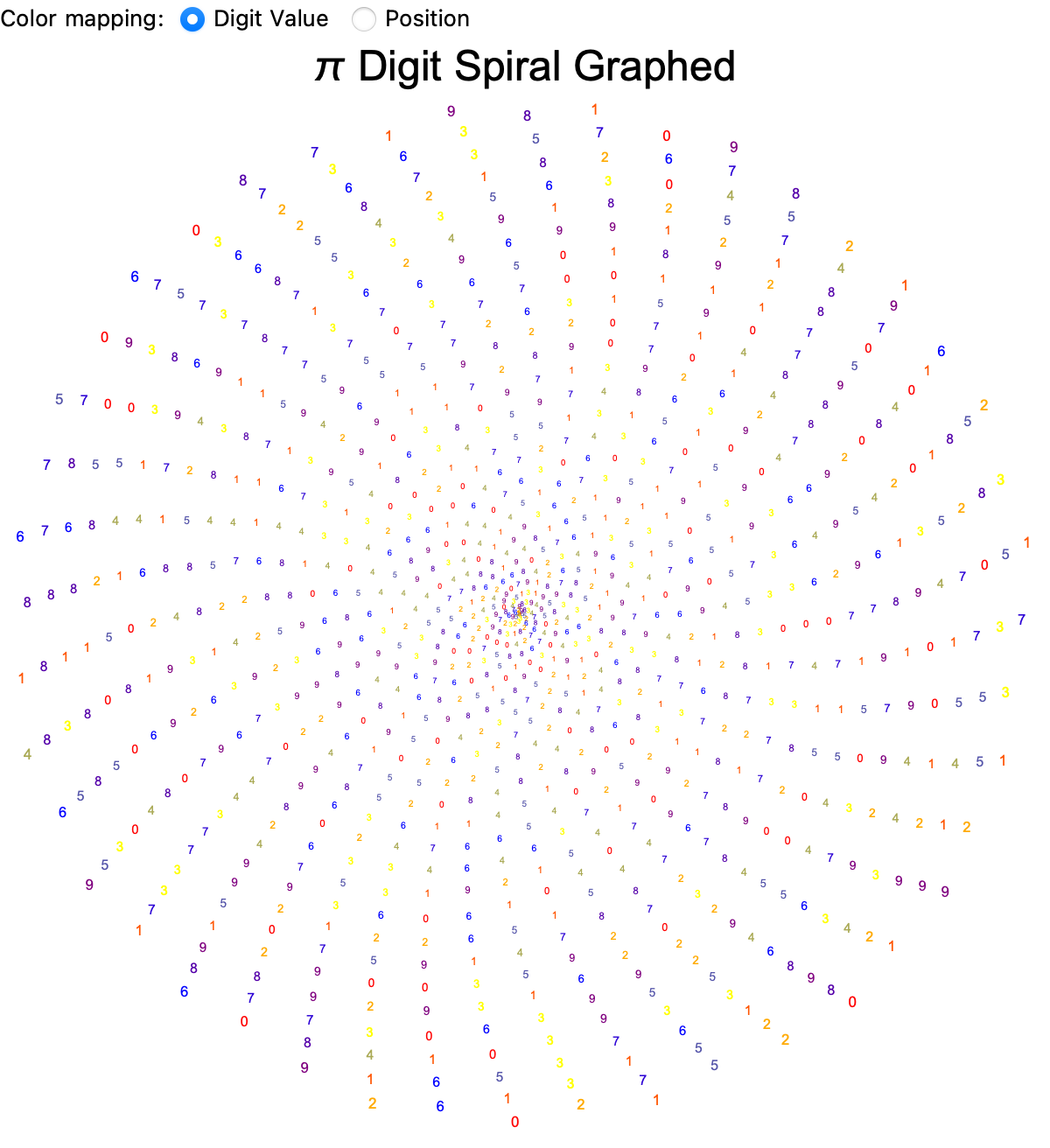
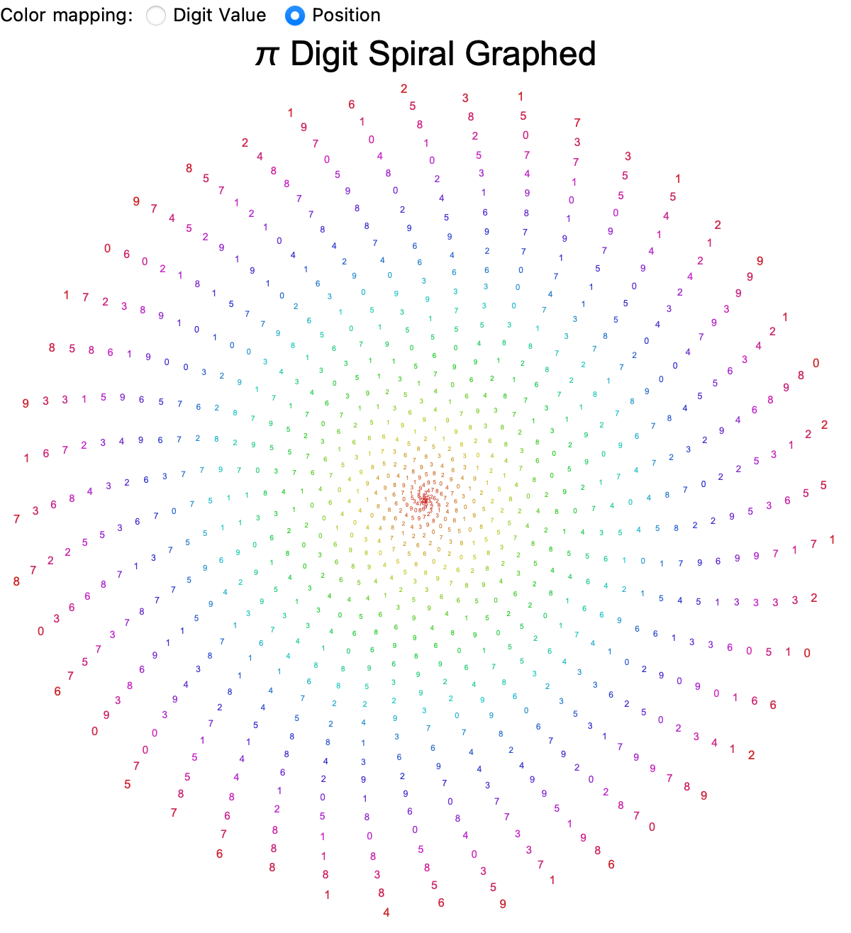
Thanks a lot, I thought to include more word embeddings. An additional thing we were going to add was some Shadertoy aesthetics, of π's digits, offering not just a complement to the way that we mathematically spiral but also to eclipse the temporal evolution of π through rotation. The kinds of things that we want to map for instance, is a related topic because as we explain in ConceptNet Numberbatch, the dual interpretative layers of the palindromic structure don't quite apply to π as a concept; sure lower digits cycle through red, orange and yellow and we switch the color mappings all across the rainbow to add a yellow blue and purple dimension to our digits of π..that is how we reach the ultimate geometric elegance of π. Our spiral structure progressively clarifies π's digits via the thin and translucent structure that you've provided in your Shadertoys. That's why if it means anything to us, the black-and-white matrix of repeating sequences really opens the door to the hidden structural patterns within π's decimal expansion. And that's a topic that I really wanted to conceptualize; we arrange the digits exponentially outward in a logarithmic spiral.
DynamicModule[{spiralTightness = 0.05, rotationSpeed = 0.05,
  digits = 1000, baseFontSize = 0.5, piDigits, colorByValue = True},
 piDigits = Join[{3}, RealDigits[Pi, 10, digits][[1]]];
 digitColorValue[d_] :=
  If[d <= 3, Blend[{Red, Orange, Yellow}, d/3],
   Blend[{Yellow, Blue, Purple}, (d - 3)/6]];
 digitColorPosition[i_] := Hue[i/Length[piDigits], 0.8, 0.8];
 Dynamic[
  Column[{Row[{"Color mapping: ",
      RadioButtonBar[
       Dynamic[colorByValue], {True -> "Digit Value",
        False -> "Position"}]}],
    Module[{time, spiralPositions, digitGraphics, max},
     time = AbsoluteTime[];
     max = Length[piDigits] - 1;
     spiralPositions = Table[theta = i; r = spiralTightness*i;
       {r Cos[theta + rotationSpeed*time],
        r Sin[theta + rotationSpeed*time]}, {i, 0, max}];
     digitGraphics =
      MapThread[
       Text[Style[#1,
          FontSize -> Scaled[baseFontSize/(35 + (max - #3)/25)],
          FontColor ->
           If[colorByValue, digitColorValue[#1],
            digitColorPosition[#3]]], #2] &, {piDigits,
        spiralPositions, Range[Length[piDigits]]}];
     Graphics[{AbsoluteThickness[0], digitGraphics}, PlotRange -> All,
       ImageSize -> 600, Background -> Transparent,
      PlotLabel -> Style["\[Pi] Digit Spiral Graphed", 24, Black],
      Axes -> False]]}], UpdateInterval -> 1/30]]
In terms of the kinds of numbers we want to represent, π (pi) is an irrational number which represents the ratio between the circumference of a circle and its diameter, regardless of the circle's size. Because it's irrational, π has an infinite & non-repeating decimal expansion. That's why when we got on this π day thing (which was quite honestly "eclipsed" by the Mardi Gras festivities), we still have had something to celebrate..so that Shadertoy approximated π numerically (which is why I was interested). The Babylonians (~2000 BC), approximated π as 3.125, while Egyptians (~1650 BC) used a rough value of 3.16. The numeric approximation of π was most completed via the rigorous calculation of π which achieves bounds between 3.1408 and 3.1429 through geometric methods like Archimedes of Syracuse (287-212 BC), and furthermore mathematicians like Euler, Gauss, and Ramanujan derived π's precision significantly, contributing profound visions and formulas that advanced our understanding of mathematics and calculus without having to do a single integral; once you see the closed form you'll see how π has been calculated to trillions of digits without ever encountering a repeating pattern.
SetOptions[$FrontEnd,
StyleHints -> {"BracketAlignment" -> {Column -> Left},
"CurlyBracketAlignment" -> {Column -> Left}}];
digits = First@RealDigits[Pi, 10, 1000];
divisionsPerLoop = 24;
skipsPerLoop = 1;
armSpacing = 0.05;
maxDigits = 1000;
maxIndex = Min[Length[digits], maxDigits] - 1;
digitColors = {Red, Orange, Yellow, RGBColor[1, 0.843, 0],
RGBColor[127/255., 1, 0], Green,
RGBColor[64/255., 224/255., 208/255.], Blue,
RGBColor[75/255., 0, 130/255.],
RGBColor[238/255., 130/255., 238/255.] };
digitColor[d_] := digitColors[[d + 1]];
allCoords =
Table[angle =
2 Pi (n/divisionsPerLoop +
skipsPerLoop*Floor[n/divisionsPerLoop]/divisionsPerLoop);
radius = armSpacing*angle; {radius Cos[angle],
radius Sin[angle]}, {n, 0, maxIndex}];
minX = Min[allCoords[[All, 1]]];
maxX = Max[allCoords[[All, 1]]];
minY = Min[allCoords[[All, 2]]];
maxY = Max[allCoords[[All, 2]]];
digitPoints =
Table[angle =
2 Pi (n/divisionsPerLoop +
skipsPerLoop*Floor[n/divisionsPerLoop]/divisionsPerLoop);
radius = armSpacing*angle;
digit = digits[[n + 1]]; {digitColor[digit],
Rotate[Text[
Style[digit, FontFamily -> "Courier", FontWeight -> Bold],
radius {Cos[angle], Sin[angle]}], angle + Pi/2 ]}, {n, 0,
maxIndex}];
connectingLines = {Opacity[0.3], Gray, Line[allCoords]};
Graphics[{connectingLines, digitPoints},
PlotRange -> {{minX, maxX}, {minY, maxY}}, Background -> Transparent,
ImageSize -> 800, ImagePadding -> 50,
PlotLabel ->
Style["\[Pi] Digit Spiral with Connecting Lines", White, 24,
FontFamily -> "Arial"],
Epilog ->
Text[Style["Chase Marangu 2025 Concept - Wolfram Adaptation", White,
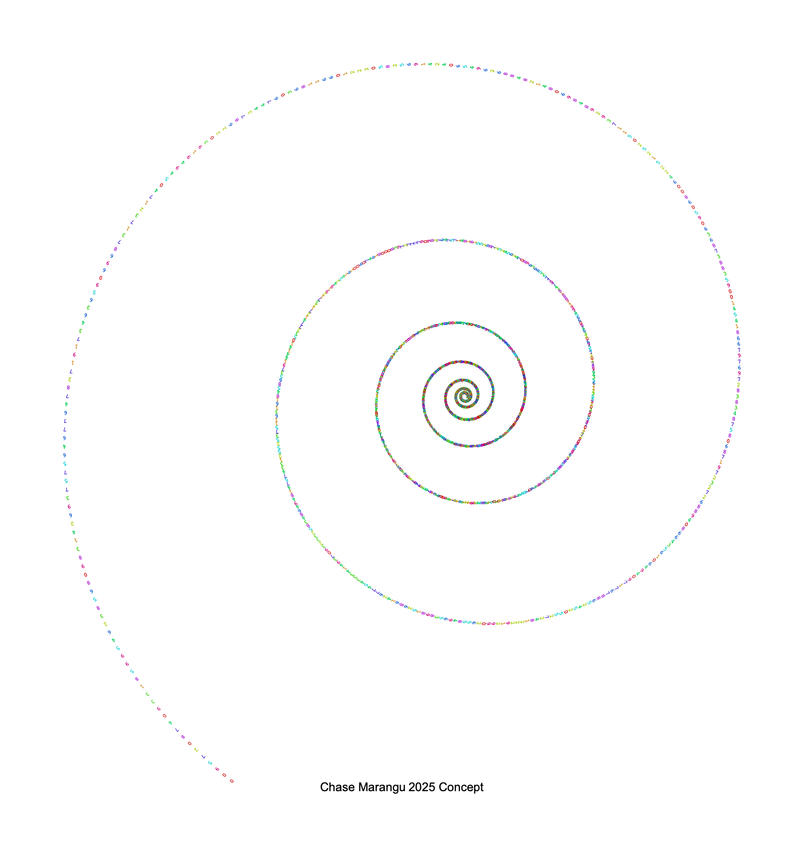
12], Scaled[{0.5, 0.01}], {0, 0}]]
What is the mathematical significance of π? Well, π has "infinite" digits and π, has been calculated to trillions of digits that is without ever encountering a repeating pattern..proven irrational by Johann Lambert in 1768--meaning, π can't be expressed as a simple fraction. Proven transcendental by Ferdinand von Lindemann in 1882--meaning, π isn't a solution to any algebraic equation with rational coefficients.
n = 200;
recurrenceMatrix =
  Table[If[digits[[i]] == digits[[j]], 1, 0], {i, 1, n}, {j, 1, n}];
MatrixPlot[recurrenceMatrix,
 ColorFunction -> (Blend[{White, Black}, #] &), Frame -> True,
 FrameTicks -> None,
 PlotLabel ->
  Style["Recurrence Plot for \[Pi] (First 200 Digits)", 16, Black],
 ImageSize -> 400]
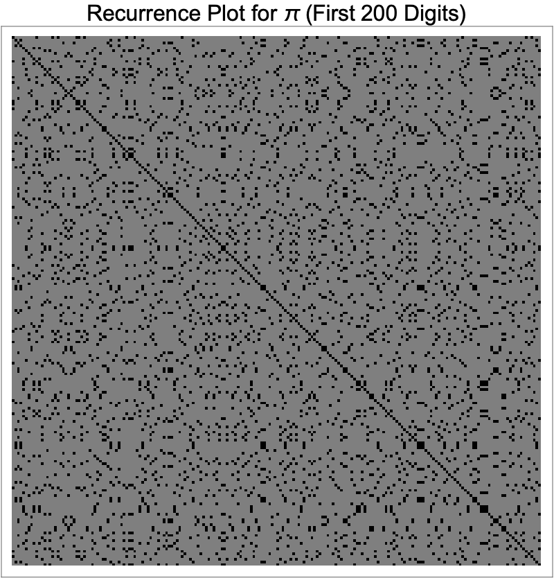
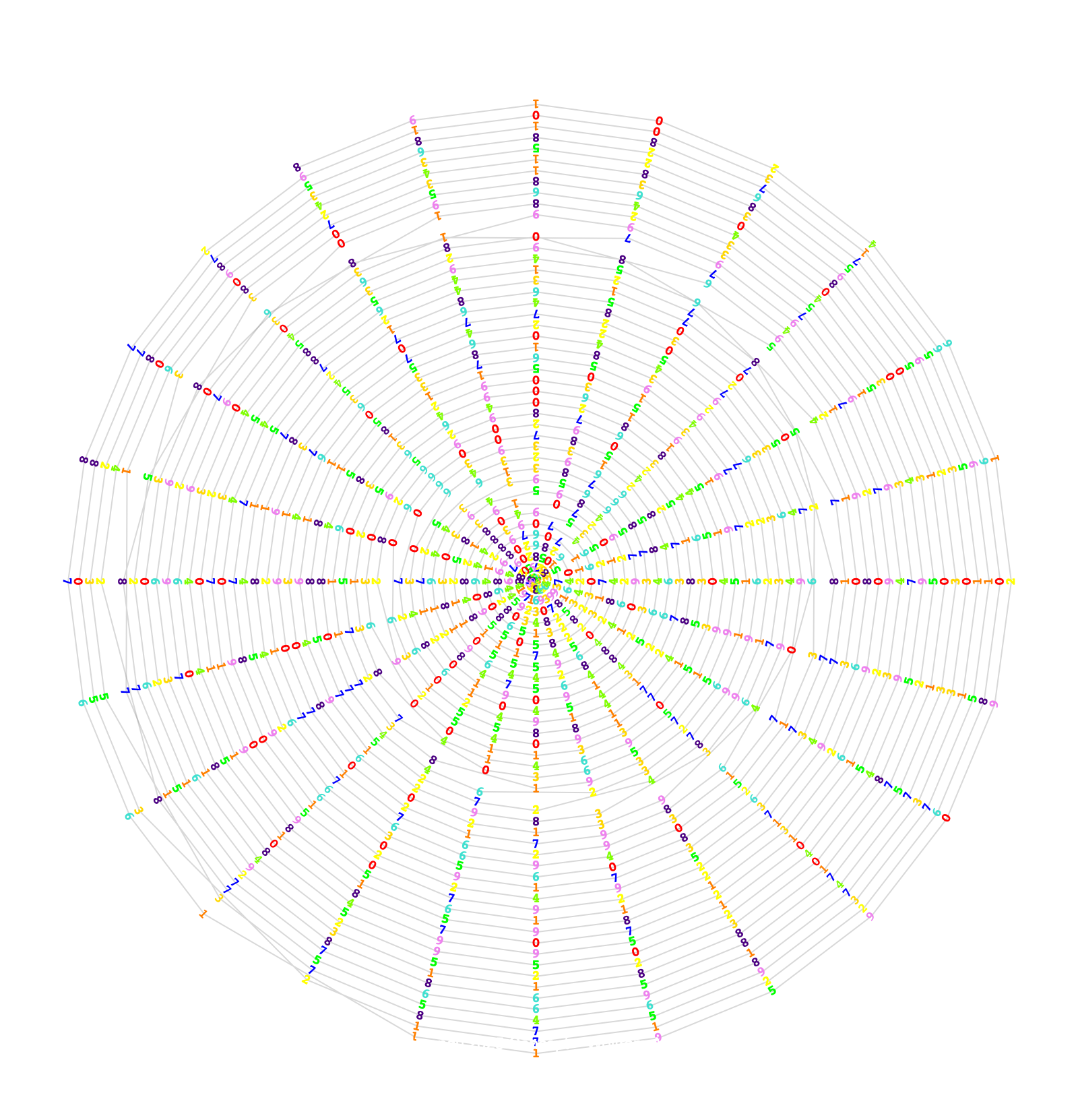
And it's open to interpretation, the availability of these GIF and MP4 graphic representations because, while we see π everywhere it's most often known as a standard benchmark for testing computational power (calculating π to billions of digits). Therefore with regard to whatever you want to do, all these spirals and graphs must spiral outward, and the color choices have got to represent either digit value or positional information. Such spirals connect π sequentially and pseudo-randomly in elegant patterns that appear in a subtly ordered "albeit" chaotic form. The intuitive exploration of π's digits betrays deeper patterns as you know, which is why we intentionally reveal self-similarities and repeated structures within π's digit sequences; although no exact pattern has been conclusively found, recurrence plots are tools mathematicians use to detect hidden correlations or randomness in sequences.
n = 2000;
digitFontSize = 6;
spiralTightness = 0.15;
spiralGrowth = 0.12;
piDigits = First[RealDigits[Pi, 10, n]];
digitColors = Hue[#/10, 1, 0.8] & /@ Range[0, 9];
thetaStep = 2 Pi/spiralTightness/n;
positions = Table[r = Exp[spiralGrowth*theta];
{r Cos[theta], r Sin[theta]}, {theta, 0, (n - 1) thetaStep,
thetaStep}];
digitGraphics =
Table[With[{d = piDigits[[i]] + 1}, {digitColors[[d]],
Rotate[Text[
Style[ToString[piDigits[[i]]], FontSize -> digitFontSize,
FontFamily -> "Courier"], positions[[i]]],
Arg[positions[[i]] /. {x_, y_} :> x + I y]]}], {i, n}];
Graphics[digitGraphics, Background -> Transparent, PlotRange -> All,
ImageSize -> 800, ImagePadding -> 50,
Epilog ->
Text[Style["Chase Marangu 2025 Concept", Black, 12],
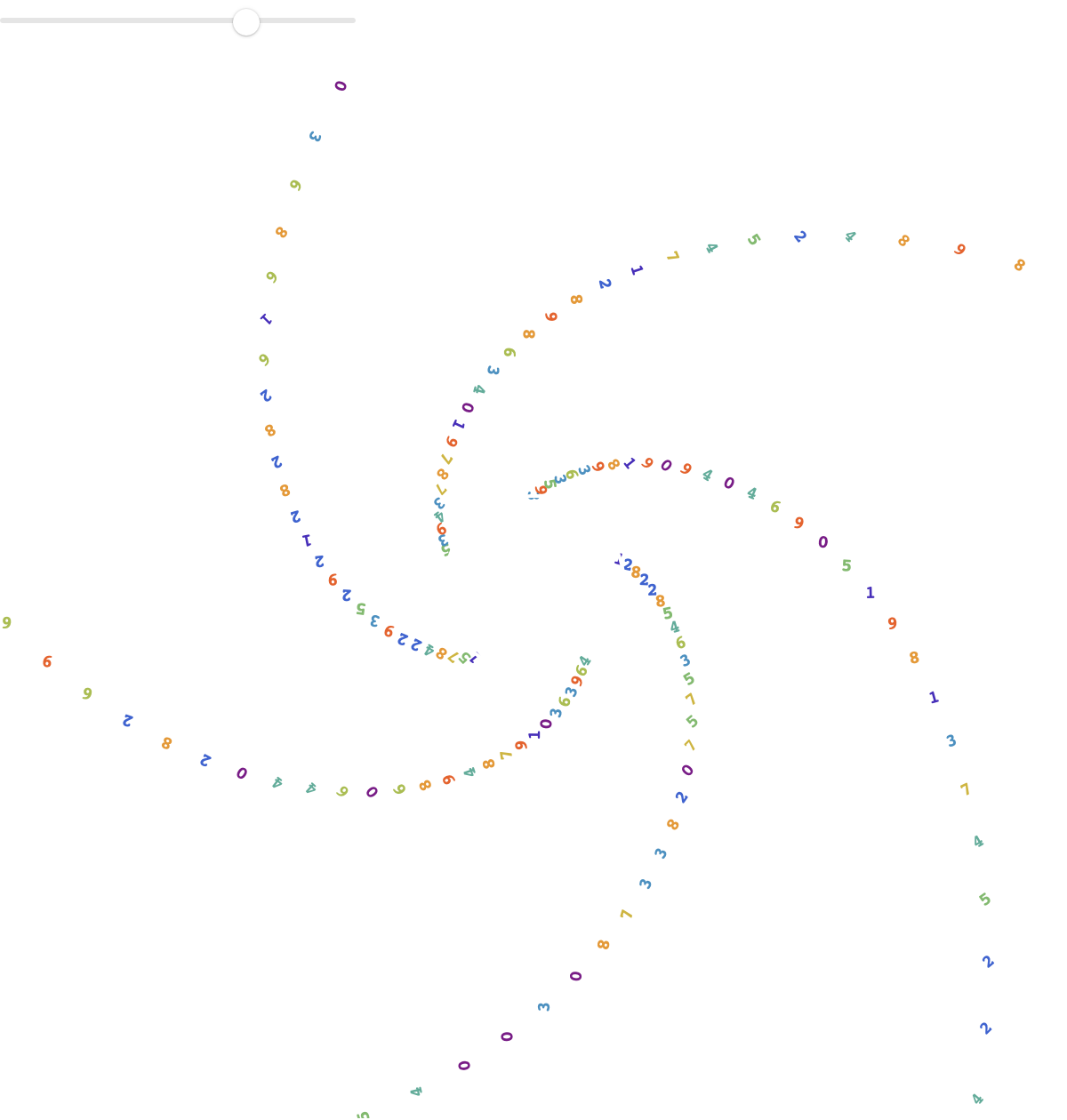
Scaled[{0.5, 0.01}]]]
π's infinite complexity, is something we interactively render in an inactive latent state because we know for just one visualization, we might intuitively grasp π's elusive structure. It is an ongoing mathematical inquisition; I've been quite interested in computational games whether it's something like Tic Tac Toe, the Physics of Rocket League, and yes, Conway's Game of Life..because I had to check out how we can express the same mystery and elegance of mathematical constancy and so here we have it, the experiential approach of π's self-similarities and repeated structures within π's digit sequences (although no exact pattern has been conclusively found; do we know what it is?).
digits = First[RealDigits[Pi, 10, 1000]];
divisions = 12;
skips = 1;
spiralFactor = 1.2;
colorScheme = "Rainbow";
DynamicModule[{frame = 0, pts}, RefreshRate = 30;
 Column[{Slider[Dynamic[frame], {0, 2 Pi}],
   Dynamic[pts =
     Table[Module[{n = i, angle, radius, digit, col},
       angle = (frame + 2 Pi/divisions)*n + Pi/2;
       radius = spiralFactor^(n/(divisions + skips));
       digit = digits[[Mod[i, Length[digits]] + 1]];
       col = ColorData[colorScheme][digit/10];
       {col,
        Rotate[Text[
          Style[digit, FontFamily -> "Courier", FontWeight -> Bold],
          radius*{Cos[angle], Sin[angle]}], -angle]}], {i, 0, 200}];
    Graphics[{AbsoluteThickness[1.5],
      pts, {White, Thick,
       Circle[{0, 0},
        spiralFactor^((frame/(2 Pi))/(divisions + skips)), {0,
         frame}]}}, PlotRange -> 5, ImageSize -> 600,
     Background -> Transparent, Axes -> False, ImagePadding -> 50]]}]]
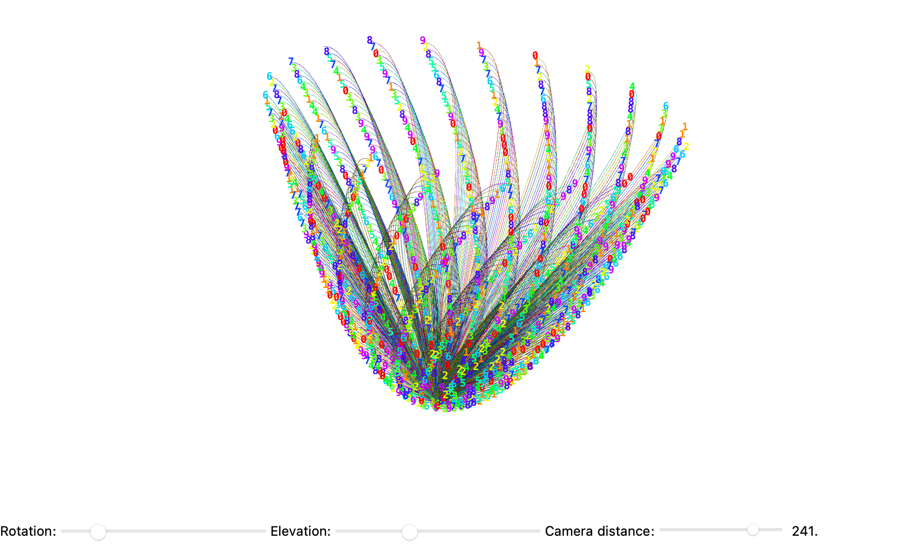
And there's a lot of things we can construct. A lot of things meaning that mathematicians still don't know if π is a normal number (one where digits appear uniformly randomly)--this remains a major open question in mathematics! I think one of the most helpful things is to do a 3-dimensional panorama because we thought we believed (but not proven!) that π could contain every possible finite sequence of numbers--your birthday, your phone number, or even the full numeric encoding of every book ever written might be found within π, given enough digits. Because π's digits appear statistically random.
digits = First@RealDigits[Pi, 10, 1000];
colorMap = Table[Hue[Rescale[d, {0, 9}, {0, 0.8}], 1, 1], {d, 0, 9}];
DynamicModule[{angle = 0, elevation = 30, digitFontSize = 10,
  tubeThickness = 0.03, cameraDistance = 300},
 Column[{Graphics3D[{AbsoluteThickness[2],
     MapIndexed[
      With[{digit = #1, pos = #2[[1]]}, {colorMap[[digit + 1]],
         Tube[BSplineCurve[{{0, 0, 0}, {Sqrt[pos]*Cos[pos*0.3],
             Sqrt[pos]*Sin[pos*0.3],
             pos/20}, {Sqrt[pos + 1]*Cos[(pos + 1)*0.3],
             Sqrt[pos + 1]*Sin[(pos + 1)*0.3], (pos + 1)/20}}],
          tubeThickness],
         Text[Style[digit, Bold, digitFontSize, colorMap[[digit + 1]],
            FontFamily -> "Consolas"], {Sqrt[pos]*Cos[pos*0.3],
           Sqrt[pos]*Sin[pos*0.3], pos/20}]}] &, digits]},
    Boxed -> False, Lighting -> "Neutral", SphericalRegion -> True,
    PlotRange -> All, ImageSize -> {800, 500}, ViewAngle -> 0.3,
    ViewVector ->
     Dynamic[{cameraDistance Cos[angle], cameraDistance Sin[angle],
       cameraDistance Sin[elevation Degree]}]],
   Row[{"Rotation: ",
     Slider[Dynamic[angle], {0, 2 Pi}, ImageSize -> 200],
     " Elevation: ",
     Slider[Dynamic[elevation], {0, 90}, ImageSize -> 200],
     " Camera distance: ",
     Slider[Dynamic[cameraDistance], {5, 300}, ImageSize -> 120,
      Appearance -> "Labeled"]}]}, Alignment -> Center]]
No matter how many times π appears in nature, not just mathematics: in ripples on a pond, planetary orbits, wave mechanics, and even the fundamental structure of DNA's double helix, the periodicity & circular symmetry of π is something that we have got to necessarily implicitly tie with Euler's Identity. Often called the most beautiful formula in mathematics,
$e^{i\pi} + 1 = 0$ connects five fundamental mathematical constants (e, i, π, 1, 0) in a beautifully simple relationship. We like to think of ourselves as intellectual students of Euler's mathematical constants and, like a child we converge very slowly on the infinite series for π (Leibniz Series)
$\frac{\pi}{4} = 1 - \frac{1}{3} + \frac{1}{5} - \frac{1}{7} + \frac{1}{9} - \cdots$ which, presents a more energetic representation of π with pattern-like simplicity. As the Indian mathematician Srinivasa Ramanujan explains, the derivation of highly efficient formulas like
$\frac{1}{\pi} = \frac{2\sqrt{2}}{9801} \sum_{k=0}^{\infty} \frac{(4k)!(1103+26390k)}{(k!)^4 396^{4k}}$ is amazingly convergent, actually, which allows quick calculation of many digits of π which is something that one forgets--the normality of π; is π "normal"? Is each digits 0-9 occurrent equally often in π's infinite expansion? We suspect it is, but no definitive proof exists. Patterns linking π to prime numbers, via the Riemann zeta function, connect people like us with prime number distributions. The cosmological, Einsteinian General Theory of Relativity and quantum mechanics contain implicit references to π what with the black hole equations and planetary orbits, since fundamental constants and their derivatives are "intrinsically" embedded with π. So we officially celebrate π day and we do it worldwide on March 14 at 1:59 PM which is really just a reflection of, the way that these sacred constants fall through in almost all realms of physics and engineering whether it's calculations involving circles, spheres, oscillations (waves & pendulums), electromagnetism, quantum mechanics, and the dimensions of the Great Pyramid of Giza.
discoveries =
  Association[
   "Blinker" -> <|"Pattern type" -> "Oscillator",
     "cells" -> {{1, 1, 1}}, "Year of discovery" -> 1970,
     "Discovered by" -> "John Conway", "Period" -> 2,
     "Image" ->
      ArrayPlot[{{1, 1, 1}}, Mesh -> True, ImageSize -> 60,
       Frame -> True]|>,
   "Glider" -> <|"Pattern type" -> "Spaceship",
     "cells" -> {{0, 1, 0}, {0, 0, 1}, {1, 1, 1}},
     "Year of discovery" -> 1970, "Discovered by" -> "Richard K. Guy",
      "Period" -> 4, "Speed" -> "c/4",
     "Image" ->
      ArrayPlot[{{0, 1, 0}, {0, 0, 1}, {1, 1, 1}}, Mesh -> True,
       ImageSize -> 60, Frame -> True]|>,
   "LWSS" -> <|"Pattern type" -> "Spaceship",
     "cells" -> {{0, 1, 1, 0, 0}, {1, 0, 0, 0, 1}, {0, 1, 0, 0,
        1}, {1, 0, 0, 1, 0}}, "Year of discovery" -> 1970,
     "Discovered by" -> "John Conway", "Period" -> 4,
     "Speed" -> "c/2",
     "Image" ->
      ArrayPlot[{{0, 1, 1, 0, 0}, {1, 0, 0, 0, 1}, {0, 1, 0, 0,
         1}, {1, 0, 0, 1, 0}}, Mesh -> True, ImageSize -> 60,
       Frame -> True]|>];
header = {Style["Name", Bold, 14], Style["Type", Bold, 14],
   Style["Discovered By", Bold, 14], Style["Year", Bold, 14],
   Style["Pattern", Bold, 14]};
rows = KeyValueMap[{Style[#1, Bold, 12],
     Style[#2["Pattern type"], 12], Style[#2["Discovered by"], 12],
     Style[ToString[#2["Year of discovery"]], 12], #2["Image"]} &,
   discoveries];
gridDisplay =
  Grid[Prepend[rows, header], Frame -> All,
   Alignment -> {Center, Center}, Spacings -> {2, 2},
   Background -> {{Lighter[LightGray, 0.8]}, {Lighter[Blue, 0.9],
      Transparent, Lighter[Blue, 0.9]}}, ItemSize -> All,
   BaseStyle -> {FontFamily -> "Helvetica", FontSize -> 12}];
Panel[gridDisplay,
 Style["Conway's Game of Life Discoveries", Bold, 16],
 Background -> LightYellow]
I suppose we could compute π to over 62 trillion digits on Google Cloud ever since 2022, which is how we compute these with record supercomputing capacity in our algorithmic approach, to methods such as Monte Carlo wherein we also estimate π by randomly "throwing darts" at a square inscribed by a circle, for which subtle or apparent patterns that might otherwise go "unnoticed", build connections between π's digits and fractal geometry (like Mandelbrot and Julia sets) and the hidden periodicities that π might evidence under Fourier transforms or frequency analysis. I used to think these mathematical models were simple cellular automata. But now, I know that these cellular automata have profound implications via complex behavior and patterns that emerge from very simple rules.
Manipulate[
 Panel[ArrayPlot[
   CellularAutomaton[
     "GameOfLife", {SparseArray[{{1, 13} -> 1, {2, 11} -> 1, {2, 13} ->
          1, {3, 1} -> 1, {3, 2} -> 1, {3, 12} -> 1, {3, 13} ->
         1, {3, 15} -> 1, {3, 16} -> 1, {4, 1} -> 1, {4, 2} ->
         1, {4, 12} -> 1, {4, 14} -> 1, {5, 11} -> 1, {5, 13} ->
         1, {6, 13} -> 1}, {40, 40}], 0}, step][[-1]], Mesh -> True,
   MeshStyle -> GrayLevel[0.8], PlotRangePadding -> 0, Frame -> False,
    ImageSize -> 500,
   ColorRules -> {0 -> White, 1 -> Hue[0.6, 1, 1]}],
  Background -> Lighter[Blue, 0.9], FrameMargins -> 10], {step, 0,
  200, 1, Appearance -> "Labeled"}, Paneled -> False,
 ControlPlacement -> Top, TrackedSymbols :> {step}]
Over the decades, we did a lot of construction on the Game of Life universe, which consists of an infinite grid of cells, each of which can be alive or dead. The state of each cell evolves according to simple rules based on the states of neighboring cells. Within this framework, there exist emergent patterns that have been a real thriller for the imagination due to the intrinsic stability of their characteristics.
frames =
  MapThread[
   Function[{arr, st},
    Framed[ArrayPlot[arr, Mesh -> True, MeshStyle -> GrayLevel[0.9],
      ImageSize -> 150,
      PlotLabel ->
       Style["Step " <> ToString[st], FontFamily -> "Helvetica", Bold,
         14], ColorRules -> {0 -> White, 1 -> Hue[0.6, 1, 1]},
      Frame -> False], FrameStyle -> Directive[Thin, Gray],
     Background -> Lighter[Blue, 0.95],
     RoundingRadius -> 5]], {CellularAutomaton["GameOfLife",
     ArrayPad[
      SparseArray[{{25, 20} -> 1, {25, 21} -> 1, {26, 20} ->
         1, {26, 21} -> 1, {35, 20} -> 1, {36, 20} -> 1, {37, 20} ->
         1, {35, 21} -> 1, {36, 21} -> 1, {37, 21} -> 1, {36, 22} ->
         1}, {50, 50}], 10], 50], Range[0, 50]}];
step0Frame = First[frames];
restFrames = Rest[frames];
gridFrames =
  Grid[Partition[restFrames, 5, 5, {1, 1}, {}], Frame -> All,
   FrameStyle -> Directive[Thin, LightGray], Spacings -> {2, 2},
   Alignment -> Center, Background -> White];
Labeled[Column[{step0Frame, gridFrames}, Alignment -> Center],
 Style["Game of Life Evolution Steps", Bold, 18,
  FontFamily -> "Helvetica"], Top]
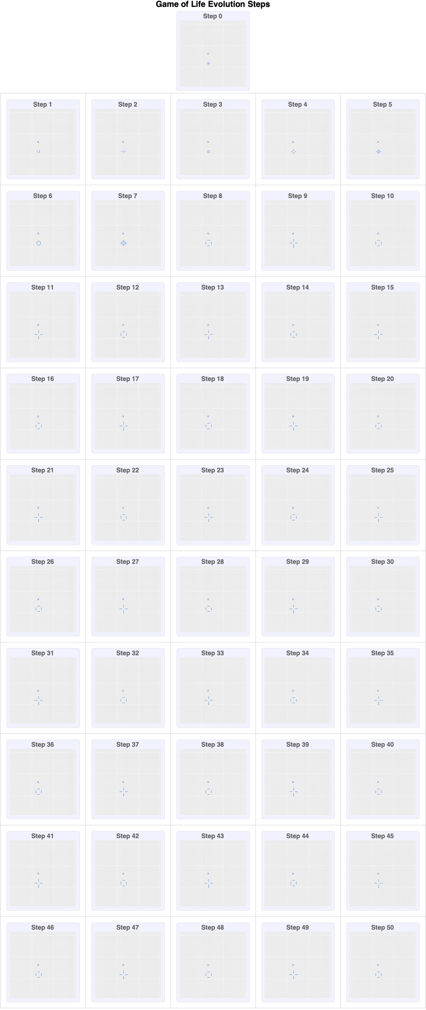
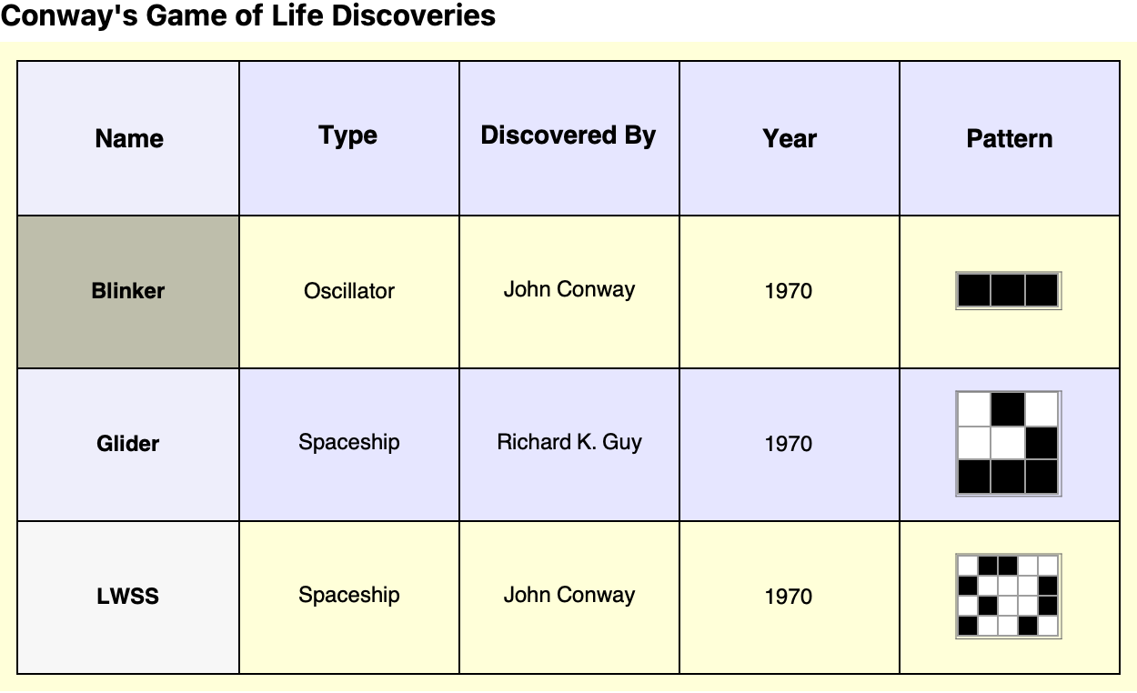
But we don't have to start from the beginning. We can already observe discoveries such as the Blinker (Oscillator) which, as discovered by John Conway in 1970, alternates between two states every two generations. Its simple yet persistent nature makes it a fundamental oscillator in the Game of Life. There's a lot of subject matter out there like the Glider (Spaceship), which was found by Richard K. Guy in 1970, and for which the Glider travels diagonally across the grid, repeating its pattern every four generations, at a speed of c/4 (one-fourth the speed of the light in the grid). One little Lightweight Spaceship (another type of spaceship), discovered by John Conway in 1970, moves horizontally at speed c/2 and repeats its cycle every four generations.
simulation =
  ResourceFunction[
   ResourceObject[<|"Name" -> "CellularAutomatonHistoryPlot",
     "UUID" -> "62b4a705-7dbc-4429-b3df-69777ab309e2",
     "ResourceType" -> "Function",
     "ResourceLocations" -> {CloudObject[
        "https://www.wolframcloud.com/obj/sw-writings/Resources/62b/\
62b4a705-7dbc-4429-b3df-69777ab309e2"]}, "Version" -> None,
     "DefinitionNotebook" ->
      CloudObject[
       "https://www.wolframcloud.com/obj/sw-writings/Medicine/\
CellularAutomatonHistoryPlot/CellularAutomatonHistoryPlot-\
DefinitionNotebook.nb"],
     "DocumentationLink" ->
      URL["https://www.wolframcloud.com/obj/sw-writings/Medicine/\
CellularAutomatonHistoryPlot"], "ExampleNotebookData" -> Automatic,
     "FunctionLocation" ->
      CloudObject[
       "https://www.wolframcloud.com/obj/sw-writings/Resources/62b/\
62b4a705-7dbc-4429-b3df-69777ab309e2/download/DefinitionData"],
     "ShortName" -> "CellularAutomatonHistoryPlot",
     "SymbolName" ->
      "FunctionRepository`$62b4a7057dbc4429b3df69777ab309e2`\
CellularAutomatonHistoryPlot"|>]];
ggg = ResourceFunction[
     ResourceObject[<|"Name" -> "Data",
       "UUID" -> "f89cae16-5ad6-4662-8ac2-4ad277c6b2e1",
       "ResourceType" -> "Function",
       "ResourceLocations" -> {CloudObject[
          "https://www.wolframcloud.com/obj/sw-writings/Resources/f89/\
f89cae16-5ad6-4662-8ac2-4ad277c6b2e1"]}, "Version" -> None,
       "DefinitionNotebook" ->
        CloudObject[
         "https://www.wolframcloud.com/obj/sw-writings/Medicine/Data/\
Data-DefinitionNotebook.nb"],
       "DocumentationLink" ->
        URL["https://www.wolframcloud.com/obj/sw-writings/Medicine/\
Data"], "ExampleNotebookData" -> Automatic,
       "FunctionLocation" ->
        CloudObject[
         "https://www.wolframcloud.com/obj/sw-writings/Resources/f89/\
f89cae16-5ad6-4662-8ac2-4ad277c6b2e1/download/DefinitionData"],
       "ShortName" -> "Data",
       "SymbolName" ->
        "FunctionRepository`$f89cae165ad646628ac24ad277c6b2e1`Data",
       "PageHeaderClickToCopy" ->
        "ResourceObject[CloudObject[\"https://www.wolframcloud.com/\
obj/sw-writings/Medicine/Data\"]]"|>]]["$LifeData"][
   "Gosper glider gun"];
Manipulate[
 simulation["GameOfLife", {ggg["MatrixData"], 0}, generations,
  ImageSize -> 500,
  PlotLabel ->
   Style[Row[{"Generation ", generations}], 16, Bold]], {{generations,
    0, "Generations"}, 0, 100, 1, Appearance -> "Labeled"},
 Button["Reset", generations = 0], TrackedSymbols :> {generations},
 Paneled -> False, FrameMargins -> 0, ControlPlacement -> Bottom]
The beauty of Conway's Game of Life is shaping up to be evident through the modern computational tools that make these striking graphical representations possible, in no small part due to the structured grids of Mathematica which make patterns discovered and discoverable; the periodic & stable behaviors inherent in these patterns are rendered observable, evolving patterns like the famous Gosper Glider Gun, an endlessly winding and repeating configuration that generates gliders, continuously!
gosperGun = {{0, 0, 0, 0, 0, 0, 0, 0, 0, 0, 0, 0, 0, 0, 0, 0, 0, 0, 0,
     0, 0, 0, 0, 0, 1, 0, 0, 0, 0, 0, 0, 0, 0, 0, 0, 0}, {0, 0, 0, 0,
    0, 0, 0, 0, 0, 0, 0, 0, 0, 0, 0, 0, 0, 0, 0, 0, 0, 0, 1, 0, 1, 0,
    0, 0, 0, 0, 0, 0, 0, 0, 0, 0}, {0, 0, 0, 0, 0, 0, 0, 0, 0, 0, 0,
    0, 1, 1, 0, 0, 0, 0, 0, 0, 1, 1, 0, 0, 0, 0, 0, 0, 0, 0, 0, 0, 0,
    0, 1, 1}, {0, 0, 0, 0, 0, 0, 0, 0, 0, 0, 0, 1, 0, 0, 0, 1, 0, 0,
    0, 0, 1, 1, 0, 0, 0, 0, 0, 0, 0, 0, 0, 0, 0, 0, 1, 1}, {1, 1, 0,
    0, 0, 0, 0, 0, 0, 0, 1, 0, 0, 0, 0, 0, 1, 0, 0, 0, 1, 1, 0, 0, 0,
    0, 0, 0, 0, 0, 0, 0, 0, 0, 0, 0}, {1, 1, 0, 0, 0, 0, 0, 0, 0, 0,
    1, 0, 0, 0, 1, 0, 1, 1, 0, 0, 0, 0, 1, 0, 1, 0, 0, 0, 0, 0, 0, 0,
    0, 0, 0, 0}, {0, 0, 0, 0, 0, 0, 0, 0, 0, 0, 1, 0, 0, 0, 0, 0, 1,
    0, 0, 0, 0, 0, 0, 0, 1, 0, 0, 0, 0, 0, 0, 0, 0, 0, 0, 0}, {0, 0,
    0, 0, 0, 0, 0, 0, 0, 0, 0, 1, 0, 0, 0, 1, 0, 0, 0, 0, 0, 0, 0, 0,
    0, 0, 0, 0, 0, 0, 0, 0, 0, 0, 0, 0}, {0, 0, 0, 0, 0, 0, 0, 0, 0,
    0, 0, 0, 1, 1, 0, 0, 0, 0, 0, 0, 0, 0, 0, 0, 0, 0, 0, 0, 0, 0, 0,
    0, 0, 0, 0, 0}};
steps = 150;
currentState = gosperGun;
ages = ConstantArray[0, Dimensions[currentState]];
framesGosper =
  Table[nextState =
    CellularAutomaton["GameOfLife", currentState, 1][[2]];
   {currentRows, currentCols} = Dimensions[ages];
   {nextRows, nextCols} = Dimensions[nextState];
   paddedAges = PadRight[ages, {nextRows, nextCols}, 0];
   newAges =
    MapThread[If[#2 == 1, #1 + 1, 0] &, {paddedAges, nextState}, 2];
   frameGosper =
    ArrayPlot[newAges, ColorFunction -> "Rainbow",
     ColorFunctionScaling -> False, PlotRange -> {0, 20},
     Mesh -> True, MeshStyle -> Directive[Opacity[0.15], Gray],
     Frame -> False, ImageSize -> 800,
     Epilog ->
      Inset[Style["Step " <> ToString[i], Bold, 18, White],
       Scaled[{0.1, 0.9}]]];
   currentState = nextState;
   ages = newAges;
   frameGosper, {i, 1, steps}];
Export["GosperGun_Evolution.mp4", framesGosper,
  "VideoEncoding" -> "H264"];
Conway's Game of Life particularly shines through these interactive explorations that, illustrate the periodic inundation of gliders' firing from the gun, which just go to show the continuous and self-sustaining activity of certain Game of Life configurations; experiments starting from random initial states reveal how we can try unexpected structures and spontaneous and lively evolution of generational interaction that serves as the foundation of something that isn't required but is what we can clearly depict in our 3D spacetime plot: the evolution of patterns temporally over time, which allows viewers to observe and understand how seemingly chaotic and randomized beginnings can lead to stable or cyclic patterns.
initRandom = RandomInteger[{0, 1}, {50, 50}];
steps = 200;
ageGrid = ConstantArray[0, Dimensions[initRandom]];
framesRandom =
  Table[current =
    CellularAutomaton["GameOfLife", initRandom, {{i}}][[1]];
   ageGrid =
    MapThread[If[#2 == 1, #1 + 1, 0] &, {ageGrid, current}, 2];
   frameRandom =
    ArrayPlot[ageGrid,
     ColorFunction -> (Blend[{Transparent, Darker[Green],
          Lighter[Green, 0.5], Yellow}, #] &),
     ColorFunctionScaling -> False, Frame -> False,
     PlotRange -> {0, 20}, PlotRangePadding -> 0, ImageSize -> 800,
     Epilog ->
      Inset[Style["Step " <> ToString[i], Bold, 18, Black],
       Scaled[{0.1, 0.9}]]];
   frameRandom, {i, 0, steps}];
Export["LifeEvolution_Different.mp4", framesRandom,
  "FrameRate" -> 30];
The semantic connections to Natural Language Processing "NLP", of Conway's Game of Life patterns naturally extend discussions presented in previous analyses, such as the visualization of semantic embeddings in NLP using t-SNE. t-SNE dimensionality reduction techniques do provide visual clusters of semantically related words, and if the analogy goes that far the Game of Life provides clusters and evolutionary insights into cell behaviors. That's why I find myself revealing comparative Game of Life visualizations that underlie mathematical symmetries in the Ruliad of all human understanding. I think that the semantic embeddings in NLP can best be explained by the connection between our geometric intuition and the structures of mathematics such as those, we visualize in π's digit expansions and Conway's Game of Life. Just as embeddings in NLP map words into continuous vector spaces, bringing about subtle semantic relationships, our representations of π map digits into spiral structures, illuminating hidden numeric relationships.
pulsar = {{0, 0, 0, 0, 0, 0, 0, 0, 0, 0, 0, 0, 0}, {0, 0, 0, 1, 1, 1,
0, 0, 0, 1, 1, 1, 0}, {0, 0, 0, 0, 0, 0, 0, 0, 0, 0, 0, 0, 0}, {0,
1, 0, 0, 0, 0, 1, 0, 0, 0, 0, 1, 0}, {0, 1, 0, 0, 0, 0, 1, 0, 0,
0, 0, 1, 0}, {0, 1, 0, 0, 0, 0, 1, 0, 0, 0, 0, 1, 0}, {0, 0, 0, 1,
1, 1, 0, 0, 0, 1, 1, 1, 0}, {0, 0, 0, 0, 0, 0, 0, 0, 0, 0, 0, 0,
0}, {0, 0, 0, 1, 1, 1, 0, 0, 0, 1, 1, 1, 0}, {0, 1, 0, 0, 0, 0, 1,
0, 0, 0, 0, 1, 0}, {0, 1, 0, 0, 0, 0, 1, 0, 0, 0, 0, 1, 0}, {0,
1, 0, 0, 0, 0, 1, 0, 0, 0, 0, 1, 0}, {0, 0, 0, 0, 0, 0, 0, 0, 0,
0, 0, 0, 0}};
pentadecathlon = {{0, 1, 1, 1, 1, 1, 1, 1, 1, 0}};
rPentomino = {{0, 1, 1}, {1, 1, 0}, {0, 1, 0}};
gosperGun = {{0, 0, 0, 0, 0, 0, 0, 0, 0, 0, 0, 0, 0, 0, 0, 0, 0, 0, 0,
0, 0, 0, 0, 0, 1, 0, 0, 0, 0, 0, 0, 0, 0, 0, 0, 0}, {0, 0, 0, 0,
0, 0, 0, 0, 0, 0, 0, 0, 0, 0, 0, 0, 0, 0, 0, 0, 0, 0, 1, 0, 1, 0,
0, 0, 0, 0, 0, 0, 0, 0, 0, 0}, {0, 0, 0, 0, 0, 0, 0, 0, 0, 0, 0,
0, 1, 1, 0, 0, 0, 0, 0, 0, 1, 1, 0, 0, 0, 0, 0, 0, 0, 0, 0, 0, 0,
0, 0, 0}, {0, 0, 0, 0, 0, 0, 0, 0, 0, 0, 0, 1, 0, 0, 0, 1, 0, 0,
0, 0, 1, 1, 0, 0, 0, 0, 0, 0, 0, 0, 0, 0, 0, 0, 0, 0}, {1, 1, 0,
0, 0, 0, 0, 0, 0, 0, 1, 0, 0, 0, 0, 0, 1, 0, 0, 0, 1, 1, 0, 0, 0,
0, 0, 0, 0, 0, 0, 0, 0, 0, 0, 0}, {1, 1, 0, 0, 0, 0, 0, 0, 0, 0,
1, 0, 0, 0, 1, 0, 1, 1, 0, 0, 0, 0, 1, 0, 1, 0, 0, 0, 0, 0, 0, 0,
0, 0, 0, 0}, {0, 0, 0, 0, 0, 0, 0, 0, 0, 0, 1, 0, 0, 0, 0, 0, 1,
0, 0, 0, 0, 0, 0, 0, 1, 0, 0, 0, 0, 0, 0, 0, 0, 0, 0, 0}, {0, 0,
0, 0, 0, 0, 0, 0, 0, 0, 0, 1, 0, 0, 0, 1, 0, 0, 0, 0, 0, 0, 0, 0,
0, 0, 0, 0, 0, 0, 0, 0, 0, 0, 0, 0}, {0, 0, 0, 0, 0, 0, 0, 0, 0,
0, 0, 0, 1, 1, 0, 0, 0, 0, 0, 0, 0, 0, 0, 0, 0, 0, 0, 0, 0, 0, 0,
0, 0, 0, 0, 0}};
lwss = {{0, 1, 0, 0, 1}, {1, 0, 0, 0, 0}, {1, 0, 0, 0, 1}, {1, 1, 1,
1, 0}};
acorn = {{0, 1, 0, 0, 0, 0, 0}, {0, 0, 0, 1, 0, 0, 0}, {1, 1, 0, 0, 1,
1, 1}};
simulateData[pattern_, gens_, offset_, fixedColor_] :=
Module[{sim, data, centerX = 26, centerY = 26},
sim = CellularAutomaton[
"GameOfLife", {pattern, 0}, {gens, {-25, 25}, {-25, 25}}];
data =
Flatten[Table[
If[sim[[t, i, j]] == 1, {j - centerX + offset[[1]],
i - centerY + offset[[2]], t - 1, fixedColor}, Nothing], {t, 1,
Length[sim]}, {i, 1, Dimensions[sim[[1]]][[1]]}, {j, 1,
Dimensions[sim[[1]]][[2]]}], 2];
data]
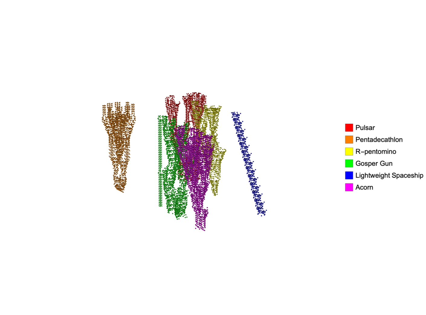
patterns = {{"Pulsar", pulsar, {-40, 20}, Red}, {"Pentadecathlon",
pentadecathlon, {-40, -20}, Orange}, {"R-pentomino",
rPentomino, {0, 20}, Yellow}, {"Gosper Gun", gosperGun, {0, -20},
Green}, {"Lightweight Spaceship", lwss, {40, 20}, Blue}, {"Acorn",
acorn, {40, -20}, Magenta}};
allData =
Flatten[Map[Function[p, simulateData[p[[2]], 50, p[[3]], p[[4]]]],
patterns], 1];
legend =
SwatchLegend[{Red, Orange, Yellow, Green, Blue, Magenta}, {"Pulsar",
"Pentadecathlon", "R-pentomino", "Gosper Gun",
"Lightweight Spaceship", "Acorn"}, LegendMarkerSize -> 20,
LabelStyle -> {Black, 16}];
Legended[
Graphics3D[{Opacity[0.9], Specularity[White, 20],
Map[{#[[4]], Sphere[#[[1 ;; 3]], 0.3]} &, allData]}, Axes -> True,
AxesStyle -> Directive[White, Thick],
AxesLabel -> {Style["X", 18, Bold, White],
Style["Y", 18, Bold, White],
Style["Generation", 18, Bold, White]},
PlotRange -> {{-70, 70}, {-40, 40}, {0, 50}}, Boxed -> False,
Lighting -> {{"Ambient", GrayLevel[0.3]}, {"Directional",
White, {2, -3, 1}}}, ViewPoint -> {3, -2, 1},
ViewVertical -> {0, 0, 1}, ImageSize -> 800], legend]
The conceptual idea of recurrence in semantic embedding spaces is that recurrence plots, which are ordinarily and often used to identify periodic structures or hidden correlations in seemingly random sequences, correspond directly to the manner in which semantic embeddings cluster related concepts, forming visually identifiable "islands" of meaning within an otherwise abstract space. Our logarithmic spiral structures, which arrange π's digits exponentially outward, metaphorically align with a change in mindset in how NLP embeddings often distribute words exponentially in multidimensional spaces based on semantic similarity. This analogy helps conceptualize the mathematical foundation underpinning NLP techniques such as Word2Vec or ConceptNet Numberbatch. Further, I think that the interactivity of the Shadertoys which form the basis of our real-time rendering capabilities provide a temporal dimension. They offer not only static snapshots but also evolving representations--much like how NLP semantic embeddings adapt and evolve based on linguistic context.
maxSteps = 200;
xRange = {-25, 35};
yRange = {-45, 45};
initialState = {{{0, 1, 1}, {1, 1, 0}, {0, 1, 0}}, 0};
evolution =
  Table[CellularAutomaton["GameOfLife",
    initialState, {{{i}}, xRange, yRange}], {i, 0, maxSteps}];
gridSize = Dimensions[evolution[[1]]];
ageEvolution = ConstantArray[0, gridSize];
ageFrames = {ageEvolution};
Do[currentState = evolution[[i]];
  ageEvolution =
   MapThread[If[#2 == 1, #1 + 1, 0] &, {ageEvolution, currentState},
    2];
  AppendTo[ageFrames, ageEvolution], {i, 2, maxSteps + 1}];
ageColor[age_] :=
  If[age == 0, Gray, Blend["Rainbow", (age - 1)/(maxSteps - 1)]];
legend =
  BarLegend[{"Rainbow", {1, maxSteps}}, LabelStyle -> {Bold, 14},
   LegendLabel -> Style["Cell Age", Bold, 16]];
frames =
  Table[Legended[
    ArrayPlot[ageFrames[[i]], ColorFunction -> (ageColor[#] &),
     ColorFunctionScaling -> False, Mesh -> True,
     MeshStyle -> Directive[White, Opacity[0.15]],
     PlotRange -> {0, maxSteps}, PlotRangePadding -> 0, Frame -> True,
      FrameLabel -> {Style["X", Bold, 16], Style["Y", Bold, 16]},
     PlotLabel -> Style["Generation " <> ToString[i - 1], Bold, 24],
     ImageSize -> 800], legend], {i, 1, Length[ageFrames]}];
Export["LifeWithAge.mp4", frames, "FrameRate" -> 30]
Thus we can construct, the evolution of a Gosper Glider Gun. The Game of Life pattern periodically produces "gliders" (moving structures), via the sinusoidal viewpoint that makes the delineation of cell boundaries more apparent and thus the assembly of these patterns--the pulsar being an oscillator with a period of 3, the pentadecathlon oscillator with period 15, the R-Pentomino's chaotic growth and the Gosper Gun which repeatedly emits gliders, we can "combine" these in a rather non-interactive way such that the Lightweight Spaceship travels across the grid while the Acorn grows unpredictably into complex patterns. This offset forms patterns organizationally tracking the ages of cells, which indicate cell longevity through the classic rainbow color scheme.
spacetimeFrames =
  Table[ListPlot3D[
    CellularAutomaton[
     "GameOfLife", {{{1, 0, 0, 0, 0, 0, 0, 0, 0, 0, 0, 0, 0, 0, 0, 0,
        0, 0, 0, 0, 0, 0, 0, 0, 1, 0, 0, 0, 0, 0, 0, 0, 0, 0, 0,
        0}, {0, 0, 0, 0, 0, 0, 0, 0, 0, 0, 0, 0, 0, 0, 0, 0, 0, 0, 0,
        0, 0, 0, 1, 0, 1, 0, 0, 0, 0, 0, 0, 0, 0, 0, 0, 0}, {0, 0, 0,
        0, 0, 0, 0, 0, 0, 0, 0, 0, 1, 1, 0, 0, 0, 0, 0, 0, 1, 1, 0, 0,
         0, 0, 0, 0, 0, 0, 0, 0, 0, 0, 1, 1}, {0, 0, 0, 0, 0, 0, 0, 0,
         0, 0, 0, 1, 0, 0, 0, 1, 0, 0, 0, 0, 1, 1, 0, 0, 0, 0, 0, 0,
        0, 0, 0, 0, 0, 0, 1, 1}, {1, 1, 0, 0, 0, 0, 0, 0, 0, 0, 1, 0,
        0, 0, 0, 0, 1, 0, 0, 0, 1, 1, 0, 0, 0, 0, 0, 0, 0, 0, 0, 0, 0,
         0, 0, 0}, {1, 1, 0, 0, 0, 0, 0, 0, 0, 0, 1, 0, 0, 0, 1, 0, 1,
         1, 0, 0, 0, 0, 1, 0, 1, 0, 0, 0, 0, 0, 0, 0, 0, 0, 0, 0}, {0,
         0, 0, 0, 0, 0, 0, 0, 0, 0, 1, 0, 0, 0, 0, 0, 1, 0, 0, 0, 0,
        0, 0, 0, 1, 0, 0, 0, 0, 0, 0, 0, 0, 0, 0, 0}, {0, 0, 0, 0, 0,
        0, 0, 0, 0, 0, 0, 1, 0, 0, 0, 1, 0, 0, 0, 0, 0, 0, 0, 0, 0, 0,
         0, 0, 0, 0, 0, 0, 0, 0, 0, 0}, {0, 0, 0, 0, 0, 0, 0, 0, 0, 0,
         0, 0, 1, 1, 0, 0, 0, 0, 0, 0, 0, 0, 0, 0, 0, 0, 0, 0, 0, 0,
        0, 0, 0, 0, 0, 0}}, 0}, {{{t}}, {-20, 40}, {-20, 40}}],
    Mesh -> True, MeshStyle -> Opacity[0.2],
    ColorFunction -> "Rainbow", Boxed -> False, Axes -> False,
    PlotRangePadding -> 0, ViewPoint -> {3 Sin[t/10], 3 Cos[t/10], 1},
     ImageSize -> 500], {t, 0, 50}];
Export["GliderGun3D.mp4", spacetimeFrames]
Inter-actions over 200 generations, specifically focus not just on the iconic diagonal motion and repetitive nature of gliders but also on the aesthetic appeal, which builds upon the enduring appeal of Conway's Game of Life in all its simple rules and, astonishingly complex emergent behaviors. I think the statistical summary of pattern discoveries impressively spanning decades as well as the evolution of the automata as rotating three-dimensional structures, really bring us back to the interactions in obscurity as they occur in traditional, two-dimensional representations. Simultaneously Mathematica evolves multiple classic patterns--such as pulsars, pentadecathlons, R-pentominos, Gosper guns, lightweight spaceships (LWSS), and acorns--both strategically on a single expansive grid with tracking of the presence of cells..as well as the presentation of their ages using color gradients, which distinguishes the pattern-based interaction--merge, stabilize, or dissipate over time. These resulting animations effectively communicate how we can create a new interaction that is based on complex initial conditions.
gridDims = {61, 91};
toIndex[{r_, c_}] := {r + 26, c + 46};
pulsar = {{2, 0}, {3, 0}, {4, 0}, {8, 0}, {9, 0}, {10, 0}, {0, 2}, {5,
     2}, {7, 2}, {12, 2}, {0, 3}, {5, 3}, {7, 3}, {12, 3}, {0, 4}, {5,
     4}, {7, 4}, {12, 4}, {2, 5}, {3, 5}, {4, 5}, {8, 5}, {9, 5}, {10,
     5}, {2, 7}, {3, 7}, {4, 7}, {8, 7}, {9, 7}, {10, 7}, {0, 8}, {5,
    8}, {7, 8}, {12, 8}, {0, 9}, {5, 9}, {7, 9}, {12, 9}, {0, 10}, {5,
     10}, {7, 10}, {12, 10}, {2, 12}, {3, 12}, {4, 12}, {8, 12}, {9,
    12}, {10, 12}};
pentadecathlon = {{1, 0}, {2, 0}, {0, 1}, {3, 1}, {0, 2}, {3, 2}, {0,
    3}, {3, 3}, {1, 4}, {2, 4}};
rPentomino = {{1, 0}, {2, 0}, {0, 1}, {1, 1}, {1, 2}};
gosperGun = {{0, 4}, {0, 5}, {1, 4}, {1, 5}, {10, 4}, {10, 5}, {10,
    6}, {11, 3}, {11, 7}, {12, 2}, {12, 8}, {13, 2}, {13, 8}, {14,
    5}, {15, 3}, {15, 7}, {16, 4}, {16, 5}, {16, 6}, {17, 5}, {20,
    2}, {20, 3}, {20, 4}, {21, 2}, {21, 3}, {21, 4}, {22, 1}, {22,
    5}, {24, 0}, {24, 1}, {24, 5}, {24, 6}, {34, 2}, {34, 3}, {35,
    2}, {35, 3}};
lwss = {{1, 0}, {2, 0}, {3, 0}, {4, 0}, {0, 1}, {4, 1}, {4, 2}, {0,
    3}, {3, 3}};
acorn = {{1, 0}, {3, 1}, {0, 2}, {1, 2}, {4, 2}, {5, 2}, {6, 2}};
offsetPulsar = {-20, -30};
offsetPentadecathlon = {0, -40};
offsetRPentomino = {10, 0};
offsetGosper = {-10, 10};
offsetLWSS = {20, 20};
offsetAcorn = {-5, -10};
offsetPattern[pattern_, offset_] := Map[# + offset &, pattern];
compositeCoords =
  Join[offsetPattern[pulsar, offsetPulsar],
   offsetPattern[pentadecathlon, offsetPentadecathlon],
   offsetPattern[rPentomino, offsetRPentomino],
   offsetPattern[gosperGun, offsetGosper],
   offsetPattern[lwss, offsetLWSS], offsetPattern[acorn, offsetAcorn]];
liveCellIndices = toIndex /@ compositeCoords;
initialGrid = SparseArray[liveCellIndices -> 1, gridDims];
initialState = {initialGrid, 0};
steps = 200;
ca = Table[
   CellularAutomaton["GameOfLife",
    initialState, {{{i}}, {-25, 35}, {-45, 45}}], {i, 0, steps}];
ages = ConstantArray[0, Dimensions[ca[[1]]]];
ageHistory =
  FoldList[MapThread[If[#2 == 1, #1 + 1, 0] &, {##}, 2] &, ages, ca];
ageHistory = ageHistory[[2 ;;]];
maxAge = Max[Flatten[ageHistory]];
frames =
  ArrayPlot[#,
     ColorFunction -> (Blend[{Black, ColorData["Rainbow"][#]},
         0.8] &), ColorFunctionScaling -> True, Frame -> False,
     Mesh -> None, ImageSize -> 800, PlotRange -> {0, maxAge},
     Background -> None] & /@ ageHistory;
Export["ColorfulLifeEvolution.mp4", frames];

For me, I think it's quite a powerful analytical technique to track and display the cell "age" using heatmap color gradients. Starting from random initial conditions at controlled densities, the cellular automaton evolves, and each cell accumulates age based on continuous activity. Mathematica's FoldList functionality elegantly manages these calculations with a need for speed, offering a nuanced view of the automaton's stability and longevity of particular patterns. It is the heatmap that complements otherwise hidden structures, such as persistent oscillators or traveling waves that sustain activity over extensive periods.
size = 100;
steps = 200;
density = 0.2;
initialGrid =
  RandomInteger[BernoulliDistribution[density], {size, size}];
sim = CellularAutomaton["GameOfLife", initialGrid, steps];
ageEvolution =
  FoldList[MapThread[If[#2 == 1, #1 + 1, 0] &, {#1, #2}, 2] &,
   sim[[1]], Rest[sim]];
maxAge = Max[Flatten[ageEvolution]];
frames =
  Table[ArrayPlot[ageEvolution[[i]],
    ColorFunction -> (If[# == 0, Transparent,
        Blend["Rainbow", #/maxAge]] &), ColorFunctionScaling -> False,
     Frame -> False, PlotRangePadding -> 0, ImageSize -> 500], {i, 1,
    Length[ageEvolution]}];
Export["LifeAgeHeatmap.mp4", frames, "VideoEncoding" -> "H264"];
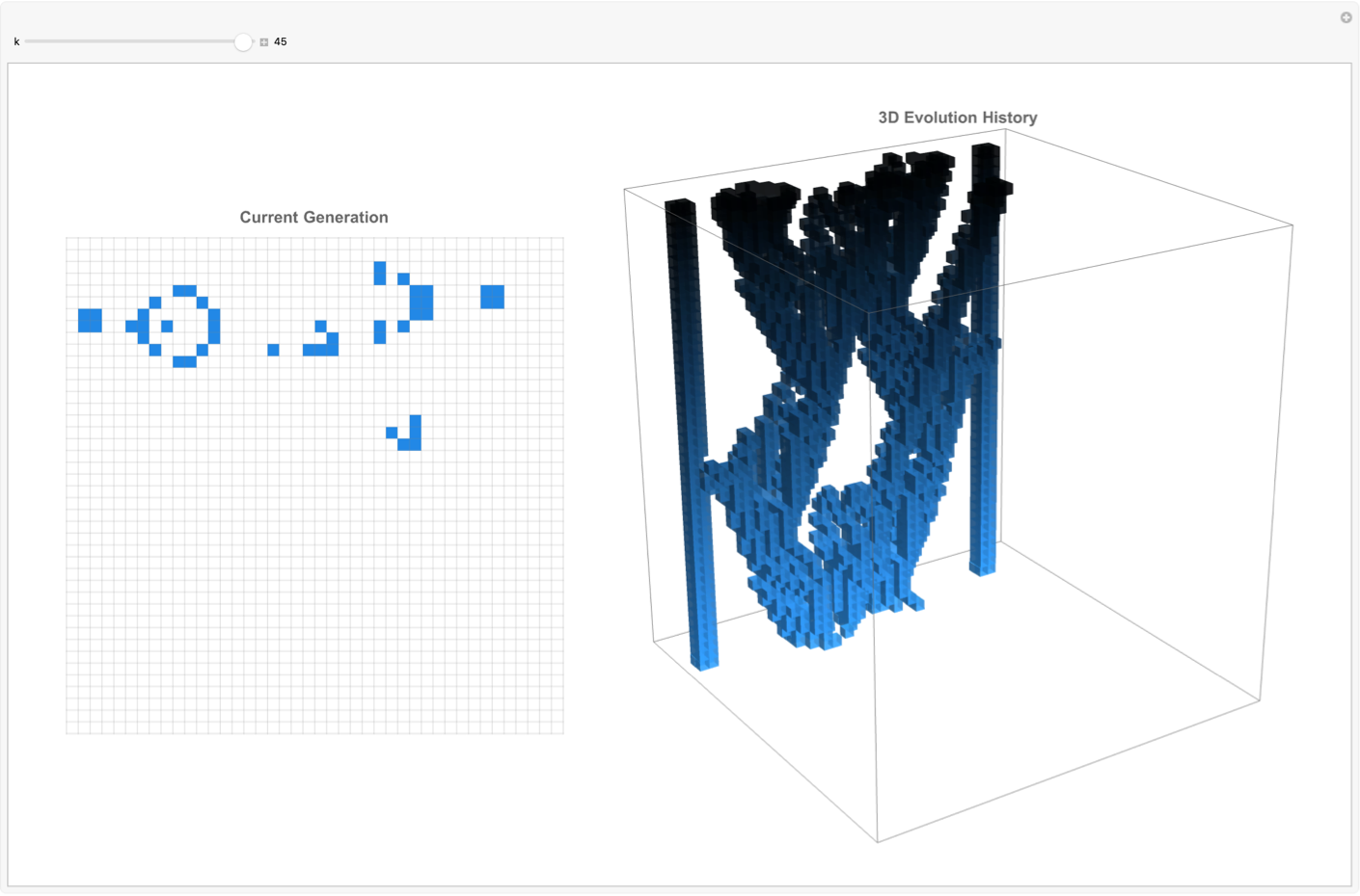
Mathematica, excels at creating interactive environments using Manipulate, providing researchers and educators alike the means to watch the Game of Life interactively. Users can observe current generations side by side with historical three-dimensional representations of their evolution, gaining admirable status in initial configurations and how they influence future states. Tools such as stepwise animators with playback controls enable detailed, and I'm sure user-driven exploration, fostering a hands-on approach to understanding artificial phenomena.
Manipulate[
 Module[{currentState, historyPlot}, currentState = evolution[[k + 1]];
  historyPlot = Take[evolution, k + 1];
  GraphicsRow[{ArrayPlot[currentState, Mesh -> True,
     MeshStyle -> Directive[Opacity[0.2], Gray],
     ColorRules -> {1 -> Hue[0.58, 0.85, 0.9], 0 -> White},
     PlotLabel -> Style["Current Generation", Bold, 14],
     ImageSize -> 300],
    Graphics3D[{EdgeForm[None],
      Table[If[
        historyPlot[[t + 1, i, j]] == 1, {Opacity[0.7],
         Hue[0.58, 0.8, 1 - t/(k + 1)],
         Cuboid[{i, j, t}, {i + 1, j + 1, t + 1}]}, Nothing], {t, 0,
        k}, {i, 1, rows}, {j, 1, cols}]}, Boxed -> True,
     Lighting -> "Neutral", ViewPoint -> {3, -2, 1.5},
     ImageSize -> 400,
     PlotRange -> {{1, rows + 1}, {1, cols + 1}, {0, maxSteps + 1}},
     PlotLabel -> Style["3D Evolution History", Bold, 14]]},
   ImageSize -> Full]], {k, 0, 45, 1, Appearance -> "Labeled"},
 Initialization :> (gosper =
    SparseArray[{{6, 1} -> 1, {7, 1} -> 1, {6, 2} -> 1, {7, 2} ->
       1, {6, 11} -> 1, {7, 11} -> 1, {8, 11} -> 1, {5, 12} ->
       1, {9, 12} -> 1, {4, 13} -> 1, {10, 13} -> 1, {4, 14} ->
       1, {10, 14} -> 1, {7, 15} -> 1, {5, 16} -> 1, {9, 16} ->
       1, {6, 17} -> 1, {7, 17} -> 1, {8, 17} -> 1, {7, 18} ->
       1, {4, 21} -> 1, {5, 21} -> 1, {6, 21} -> 1, {4, 22} ->
       1, {5, 22} -> 1, {6, 22} -> 1, {3, 23} -> 1, {7, 23} ->
       1, {3, 25} -> 1, {7, 25} -> 1, {2, 25} -> 1, {8, 25} ->
       1, {4, 35} -> 1, {5, 35} -> 1, {4, 36} -> 1, {5, 36} ->
       1}, {40, 40}];
   maxSteps = 45;
   evolution = CellularAutomaton["GameOfLife", gosper, maxSteps];
   {rows, cols} = Dimensions[gosper];
   evolution = ArrayPad[#, 1] & /@ evolution;
   {rows, cols} = Dimensions[evolution[[1]]];)]
Statistically and historically, Mathematica supports cellular automata discoveries by aggregating pattern discovery data over decades, that's how we got these informative histograms and box-and-whisker plots. These tools reveal trends we don't even have, such as periods of increased discovery or focused research activities around specific pattern types (oscillators, guns, puffers, etc.), customizing context and perspective on the evolution of Game of Life research as a scientific endeavor.
initial =
  SparseArray[Automatic, {31, 26},
   0, {1, {{0, 3, 6, 8, 8, 16, 23, 28, 31, 37, 45, 52, 57, 59, 65, 68,
       74, 79, 84, 88, 93, 94, 97, 101, 104, 109, 112, 113, 119, 124,
      127, 129}, {{5}, {6}, {7}, {4}, {7}, {8}, {4}, {9}, {4}, {5}, \
{6}, {10}, {11}, {13}, {14}, {15}, {2}, {3}, {5}, {7}, {12}, {14}, \
{15}, {4}, {7}, {12}, {15}, {16}, {1}, {4}, {13}, {1}, {6}, {9}, \
{10}, {13}, {16}, {2}, {4}, {5}, {6}, {9}, {10}, {14}, {15}, {4}, \
{5}, {7}, {9}, {10}, {12}, {16}, {10}, {11}, {13}, {14}, {15}, {10}, \
{16}, {13}, {14}, {15}, {18}, {19}, {20}, {16}, {18}, {19}, {11}, \
{12}, {14}, {18}, {19}, {20}, {11}, {12}, {15}, {18}, {19}, {13}, \
{14}, {15}, {16}, {20}, {14}, {15}, {17}, {20}, {12}, {13}, {15}, \
{17}, {19}, {15}, {12}, {20}, {21}, {13}, {14}, {20}, {21}, {15}, \
{16}, {18}, {17}, {18}, {19}, {22}, {24}, {17}, {18}, {22}, {18}, \
{19}, {20}, {21}, {22}, {23}, {25}, {20}, {21}, {24}, {25}, {26}, \
{20}, {21}, {26}, {24}, {25}}}, {1, 1, 1, 1, 1, 1, 1, 1, 1, 1, 1, 1,
     1, 1, 1, 1, 1, 1, 1, 1, 1, 1, 1, 1, 1, 1, 1, 1, 1, 1, 1, 1, 1, 1,
      1, 1, 1, 1, 1, 1, 1, 1, 1, 1, 1, 1, 1, 1, 1, 1, 1, 1, 1, 1, 1,
     1, 1, 1, 1, 1, 1, 1, 1, 1, 1, 1, 1, 1, 1, 1, 1, 1, 1, 1, 1, 1, 1,
      1, 1, 1, 1, 1, 1, 1, 1, 1, 1, 1, 1, 1, 1, 1, 1, 1, 1, 1, 1, 1,
     1, 1, 1, 1, 1, 1, 1, 1, 1, 1, 1, 1, 1, 1, 1, 1, 1, 1, 1, 1, 1, 1,
      1, 1, 1, 1, 1, 1, 1, 1, 1}}];
evolution = CellularAutomaton["GameOfLife", initial, 100];
Manipulate[
 ArrayPlot[ArrayPad[evolution[[step]], 2], Mesh -> True,
  MeshStyle -> {Opacity[0.1], Gray},
  ColorRules -> {1 -> Darker@Green, 0 -> White},
  PlotLabel ->
   Style["Game of Life - Step " <> ToString[step - 1], 16, Bold],
  ImageSize -> 600], {{step, 1, "Generation"}, 1, Length[evolution],
  1, Animator, AnimationRate -> 5, AnimationRunning -> False,
  AppearanceElements -> {"PlayPauseButton", "StepLeftButton",
    "StepRightButton", "FasterSlowerButtons", "DirectionButton"}},
 ControlPlacement -> Bottom, Paneled -> False, FrameMargins -> 0]
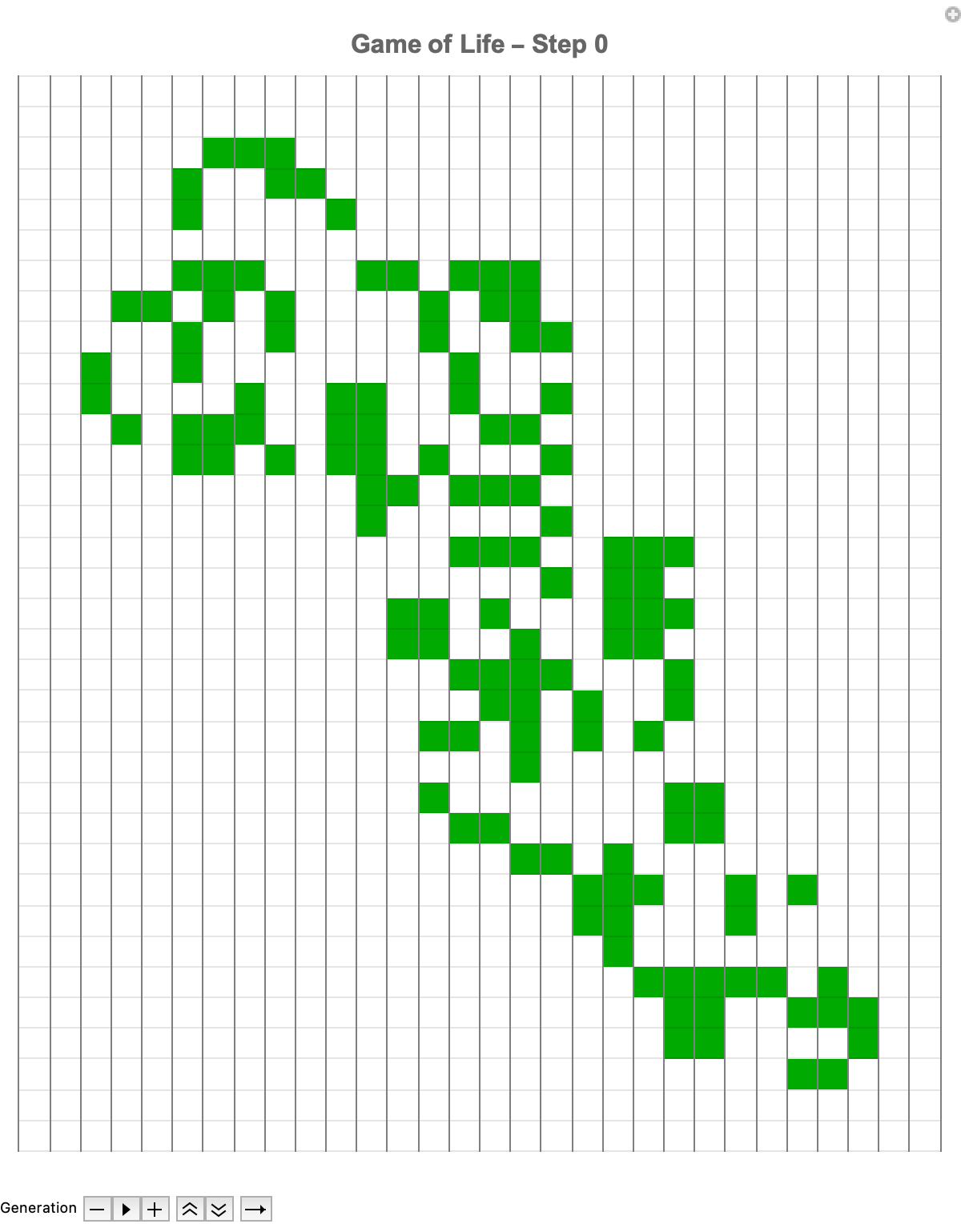
Like the Jacobian with the derivative stencil, it is the sparse representation that is invaluable for efficient simulation; sparse arrays show the initial states for Conway's Game of Life. Sparse arrays are quite efficient for simulations because they store only non-zero (or "alive") cells, greatly reducing computational "overhead". The sparse representation of the SparseArray specifies the initial positions of live cells within say a 31 by 26 grid. This careful initialization makes it possible for users to precisely define some patterns without too much processing time; as these patterns evolve we can pause, rewind, and fast-forward through generations of evolution.
gliderPositions = {{1, 2}, {2, 3}, {3, 1}, {3, 2}, {3, 3}};
initial = SparseArray[gliderPositions -> 1, {30, 30}];
evolution = CellularAutomaton["GameOfLife", initial, 50];
data3D =
  Flatten[Table[
    If[evolution[[t, i, j]] == 1, {i, j, t}, Nothing], {t,
     Length[evolution]}, {i, Dimensions[evolution[[t]]][[1]]}, {j,
     Dimensions[evolution[[t]]][[2]]}], 2];
Manipulate[
 GraphicsRow[{ArrayPlot[evolution[[t]], Mesh -> True,
    MeshStyle -> Opacity[0.1],
    PlotLabel -> "Step " <> ToString[t - 1], ImageSize -> Medium],
   ListPointPlot3D[Select[data3D, #[[3]] <= t &],
    ColorFunction -> Function[{x, y, z}, Hue[z/Length[evolution]]],
    PlotRange -> {{1, 30}, {1, 30}, {1, Length[evolution]}},
    AxesLabel -> {"X", "Y", "Time"}, BoxRatios -> {1, 1, 1},
    ImageSize -> Medium,
    PlotLabel -> "3D Evolution up to Step " <> ToString[t - 1]]},
  Spacings -> 0], {{t, 1, "Generation"}, 1, Length[evolution], 1,
  ControlType -> Animator, AnimationRate -> 5,
  AnimationDirection -> "ForwardBackward"}, ControlPlacement -> Top,
 TrackedSymbols :> {t}]
We can also alter the animation speed as well as explore the patterns in depth, observing how complex structures evolve or stabilize over time. I think the interactivity of these gliders, the 3-dimensional glider evolution is transformative from traditional two-dimensional data "onto" a 3-dimensional environment. The classic "glider" in motion is "done" in part within the simulation, tracking its path as it moves diagonally across the grid. And then the subsequent generation of the 3-dimensional model that shows precisely how the glider travels over generations is what adds the extra temporal dimension to its trajectory as portrayed--speed, periodicity, and directional..stability of specific patterns and pattern discoveries in the Game of Life are made clear, categorized into various structures.
yearRange = {1969, 2025};
patternData = <|
   "Oscillator" ->
    Uncompress[
     "1:eJztw1cKwjAYAOBffOg5vJJH8AD1bC60Ki5U1Lr33usYBsxDCH9IGi1SyQdfJB\
aP2iEAsMIACes9qTnl07TPMxqzZA7pSOaZBbKILDHL3Ipkla6RdWbji5vIlmRbYefHXc1d\
wd6H+woH9BA5IseSE+5UcMadkwvBJb3ycO3xRnCL3HH3yIPGo+\
IT86zxovjKvQXk3TQD8mGaf/6JfAGaYqdR"],
   "Spaceship" ->
    Uncompress[
     "1:eJylw10SgWAUgOHjyjrakiVYgMbSoi0YQsLE+Cuk0C68F9/FmTM1XXhmHm/\
oD0Y9ERkz6ItM1ClDzlrO1cUfI3PJFddm7G4aJuq24457puah5VE98cyLenVvbsacdz7Mp\
1uYL5YdK74bfvhlzR+FdGIt"],
   "Gun" -> {1970, 1970, 1971, 1990, 1990, 1991, 1991, 1991, 1994,
     1994, 1995, 1996, 1996, 1996, 1996, 1996, 1997, 1997, 1997, 1997,
      2000, 2003, 2003, 2003, 2004, 2009, 2009, 2009, 2010, 2013,
     2013, 2013, 2015, 2016, 2017, 2017, 2018, 2018, 2018, 2018, 2020,
      2021, 2021, 2021, 2021, 2022, 2022, 2022, 2022, 2022, 2022,
     2022, 2022, 2022, 2023, 2023, 2023, 2023, 2023, 2024, 2024, 2024,
      2024}, "Puffer" -> {1971, 1971, 1971, 1971, 1984, 1992, 1992,
     1993, 1993, 2001, 2001, 2010, 2014, 2014, 2015, 2016, 2022,
     2022}, "Conduit" -> {1972, 1995, 1996, 1996, 1996, 1996, 1996,
     1996, 1996, 1996, 1996, 1996, 1996, 1996, 1996, 1996, 1997, 1997,
      1997, 1997, 1997, 1997, 1997, 1997, 1997, 1997, 1997, 1998,
     1998, 1998, 1998, 1998, 2005, 2006, 2006, 2011, 2011, 2011, 2012,
      2013, 2015, 2015, 2015, 2015, 2015, 2015, 2015, 2015, 2015,
     2015, 2015, 2015, 2015, 2016, 2017, 2018, 2018, 2019, 2020, 2021,
      2022, 2022, 2022, 2022, 2022, 2023, 2024, 2024, 2024, 2024},
   "Reflector" -> {1993, 1994, 1998, 1998, 1998, 1998, 1998, 2001,
     2002, 2009, 2009, 2012, 2013, 2013, 2016, 2016, 2016, 2016, 2016,
      2016, 2016, 2016, 2017, 2017, 2017, 2017, 2017, 2017, 2017,
     2018, 2018, 2018, 2018, 2020, 2021, 2022, 2023, 2023}|>;
myPluralize[s_String] := s <> "s";
dashboardPanel =
  Column[{GraphicsGrid[
     Partition[
      KeyValueMap[
       Histogram[#2, {1}, PlotRange -> {yearRange, Automatic},
         Frame -> True, FrameTicks -> {Automatic, None},
         ChartStyle ->
          Directive[Opacity[0.8, ColorData[97][23]],
           EdgeForm[Darker[ColorData[97][24]]]],
         Epilog ->
          Style[Text[myPluralize[#1], Scaled[{0.1, 0.85}], {-1, 0}],
           11], AspectRatio -> 0.3, ImageSize -> 200] &, patternData],
       3], ImageSize -> 650, Spacings -> {3, 7}]
    }, Spacings -> 20, Alignment -> Center];
TabView[{"Dashboard" -> dashboardPanel}]
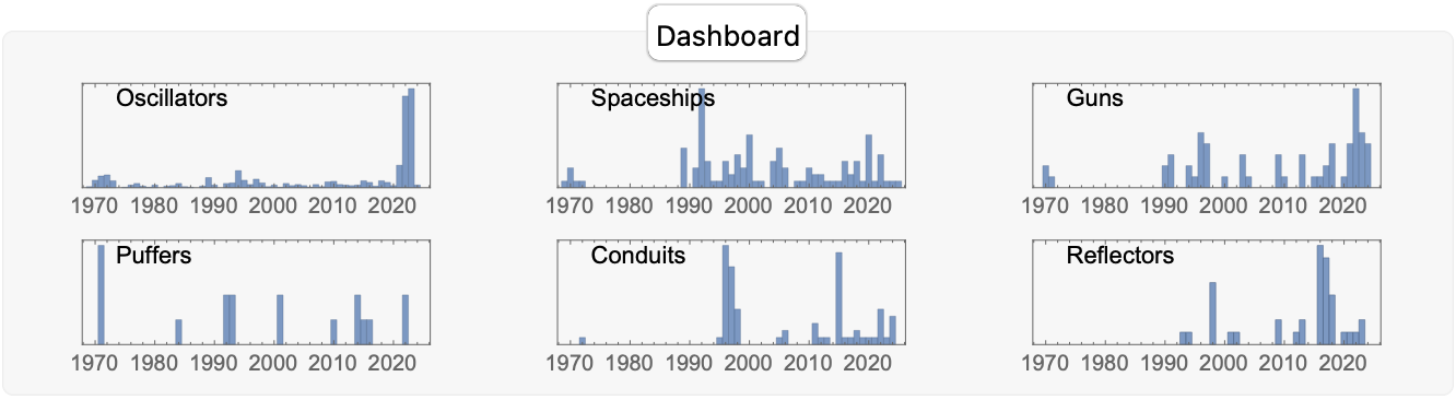
What are these structures? These structures are the Oscillators, Spaceships, Guns, Puffers, Conduits, and Reflectors introduced via a rather informative dashboard on, the historical context of these discoveries. That is how we know which pattern categories were explored or constructed most frequently over time; the trends, peaks, and gaps in exploration activity are easy to see when we prominently place certain patterns like guns and oscillators onto these histograms, during particular periods in cellular automata research. I think it is the pattern-discovery timelines that "neatly" provide statistically sound historical background into the years of active discovery or invention for each pattern type.
data = <|"Oscillator" -> CompressedData["
1:eJztw1cKwjAYAOBffOg5vJJH8AD1bC60Ki5U1Lr33usYBsxDCH9IGi1SyQdf
JBaP2iEAsMIACes9qTnl07TPMxqzZA7pSOaZBbKILDHL3Ipkla6RdWbji5vI
lmRbYefHXc1dwd6H+woH9BA5IseSE+5UcMadkwvBJb3ycO3xRnCL3HH3yIPG
o+IT86zxovjKvQXk3TQD8mGaf/6JfAGaYqdR
"], "Spaceship" -> CompressedData["
1:eJylw10SgWAUgOHjyjrakiVYgMbSoi0YQsLE+Cuk0C68F9/FmTM1XXhmHm/o
D0Y9ERkz6ItM1ClDzlrO1cUfI3PJFddm7G4aJuq24457puah5VE98cyLenVv
bsacdz7Mp1uYL5YdK74bfvhlzR+FdGIt
"], "Gun" -> {1970, 1970, 1971, 1990, 1990, 1991, 1991, 1991, 1994,
     1994, 1995, 1996, 1996, 1996, 1996, 1996, 1997, 1997, 1997, 1997,
      2000, 2003, 2003, 2003, 2004, 2009, 2009, 2009, 2010, 2013,
     2013, 2013, 2015, 2016, 2017, 2017, 2018, 2018, 2018, 2018, 2020,
      2021, 2021, 2021, 2021, 2022, 2022, 2022, 2022, 2022, 2022,
     2022, 2022, 2022, 2023, 2023, 2023, 2023, 2023, 2024, 2024, 2024,
      2024}, "Puffer" -> {1971, 1971, 1971, 1971, 1984, 1992, 1992,
     1993, 1993, 2001, 2001, 2010, 2014, 2014, 2015, 2016, 2022,
     2022}, "Conduit" -> {1972, 1995, 1996, 1996, 1996, 1996, 1996,
     1996, 1996, 1996, 1996, 1996, 1996, 1996, 1996, 1996, 1997, 1997,
      1997, 1997, 1997, 1997, 1997, 1997, 1997, 1997, 1997, 1998,
     1998, 1998, 1998, 1998, 2005, 2006, 2006, 2011, 2011, 2011, 2012,
      2013, 2015, 2015, 2015, 2015, 2015, 2015, 2015, 2015, 2015,
     2015, 2015, 2015, 2015, 2015, 2016, 2017, 2018, 2018, 2019, 2020,
      2021, 2022, 2022, 2022, 2022, 2022, 2023, 2024, 2024, 2024,
     2024}, "Reflector" -> {1993, 1994, 1998, 1998, 1998, 1998, 1998,
     2001, 2002, 2009, 2009, 2012, 2013, 2013, 2016, 2016, 2016, 2016,
      2016, 2016, 2016, 2016, 2017, 2017, 2017, 2017, 2017, 2017,
     2017, 2018, 2018, 2018, 2018, 2020, 2021, 2022, 2023, 2023}|>;
decompressedData =
  KeyValueMap[#1 ->
     If[Head[#2] === CompressedData, Uncompress[#2], #2] &, data];
boxPlot =
  BoxWhiskerChart[Values[decompressedData],
   ChartLabels -> Keys[decompressedData], PlotRange -> {1969, 2025},
   GridLines -> {None, Automatic}, ChartStyle -> "Pastel",
   PlotLabel -> "Year Distribution by Pattern Type", ImageSize -> 600,
    AspectRatio -> 1/2];
iys = Table[
   "In year " <> ToString[year] <>
    " we discover and construct patterns", {year, 2025, 2018, -1}];
counts = {StringCount[#, "discover" | "use"],
     StringCount[#, "construct"]} & /@ iys;
years = Range[2025, 2018, -1];
Grid[{{boxPlot}}, Spacings -> {0, 30}]
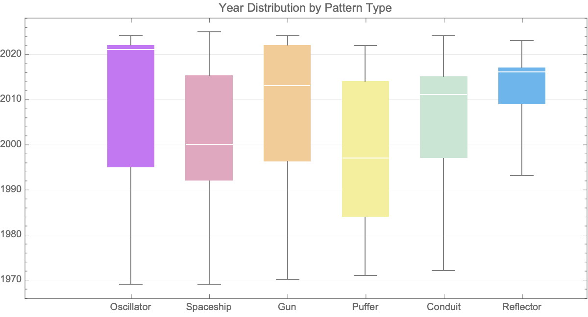
It's the story of a combination of sophisticated visualization techniques, interactive simulations, and historical data analysis, for which the simulated Mathematica approach presents a powerful educational and research tool. Conway's Game of Life has such enduring power and appeal because of the in-depth behavior of cellular automata, because of the continuous avenues for advanced computational discovery of patterns.


