Hi Bruce,
I am not quite sure whether I understand what you want to achieve, but here is an idea. Suppose you have the following tabular data:
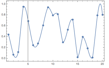
tab = Transpose[{Range[0, 20], RandomReal[1, {21}]}]
To get this into your ODE you could interpolate it:
k = Interpolation[tab]
This looks like
Show[Plot[k[t], {t, 1, 20}, Frame -> True], ListPlot[tab]]
Then you can use that in your ODE:
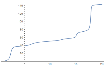
sols = NDSolve[{D[z[t], t] == 1/k[t], z[1] == 1}, z, {t, 1, 20}]
This can be plotted now:
Plot[z[t] /. sols, {t, 1, 20}]
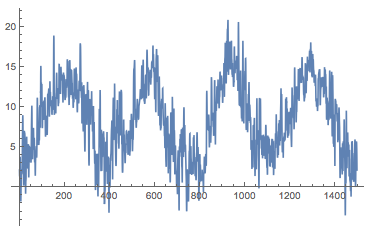
Here's an application. I want to know what the temperature of the soil in different depths is. I use the air temperature for Aberdeen (UK) where I live.
tempAberdeen = WeatherData["EGPD", "Temperature", {{2011, 1, 1}, Date[], "Day"}]["Values"];
I then fit a function to that:
f = Interpolation[Transpose[{Range[Length[tempAberdeen]] - 1, tempAberdeen}]]
Looks like this:
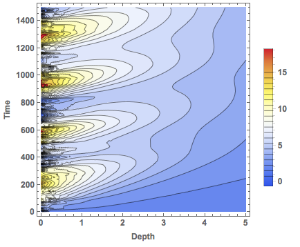
I then use the diffusion equation to see how the temperature distribution in the soil is.
f = Interpolation[Transpose[{Range[Length[tempAberdeen]] - 1, tempAberdeen}]]; sols = NDSolve[{D[[Theta][x, t], t] == 0.01* D[[Theta][x, t], {x, 2}], [Theta][0, t] == f[t], [Theta][x, 0] == f[0], D[[Theta][x, t], x] == 0 /. x -> 0}, [Theta][x, t], {x, 0, 10}, {t, 0, Length[tempAberdeen] - 1}, PrecisionGoal -> 100, MaxSteps -> Infinity, MaxStepFraction -> 1/1000.]
The temperature of the soil at the initial time is badly chosen so my result is not quite accurate, but it illustrates the idea.
ContourPlot[\[Theta][x, t] /. sols, {x, 0, 5}, {t, 0, Length[tempAberdeen]}, PlotRange -> All, PlotLegends -> True,
 Contours -> 20, FrameLabel -> {"Depth", "Time"}, LabelStyle -> Directive[Medium, Bold], ColorFunction -> "TemperatureMap"]
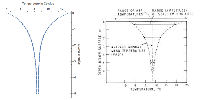
You can then represent the fluctuations at different depths and compare that to textbook knowledge:
t
empdepth =
  Join[Table[{Mean[
        Table[\[Theta][x, t] /. sols /. x -> g, {t, 1, 1000}]][[1]] +
      StandardDeviation[
        Table[\[Theta][x, t] /. sols /. x -> g, {t, 1, 1000}]][[
       1]], -g}, {g, 0, 5, 0.05}],
   Table[{Mean[
        Table[\[Theta][x, t] /. sols /. x -> g, {t, 1, 1000}]][[
       1]] + -StandardDeviation[
         Table[\[Theta][x, t] /. sols /. x -> g, {t, 1, 1000}]][[
        1]], -g}, {g, 0, 5, 0.05}]];
ListPlot[tempdepth, PlotRange -> All, AspectRatio -> 1.3, Frame -> {{False, True}, {False, True}}, FrameTicks -> All,
 FrameLabel -> {{"", "Depth in Meters"}, {"",
    "Temperature in Celsius"}}, LabelStyle -> Directive[Medium, Bold]]
You obtain the following graphic (where I have dealt with the bad initial condition, so if you run the code above you do not get exactly this):
I am aware that this answer is a kind of an over-kill, and might not even answer the question you have...
Cheers,
Marco


