Message Boards Message Boards

3
|
39963 Views
|
34 Replies
|
24 Total Likes
View groups...
Share
Share this post:

How to force Mathematica calculations in Reals domain only ?

Hi All

Maybe it's a silly question for experienced users, but I'm rather new and I'm having troubles. I need to know if there is a way to force Mathematica to work in the Reals domain.

For example, if I do

Plot[x^(1/3),{x,-10,10}]

I obtain a plot only for positive reals, For negative ones Mathematica branches to a complex root and doesn't plot it.

I know that in the past existed a package called RealOnly which did the job, but now it's obsolete.

I tried several combinations of Assumptions and so on, but couldn't figure out how to use them.

Many thanks

Stefano

34 Replies
Posted 9 years ago

Ah . . . It chooses one of the complex roots:

In[16]:= x /. Solve[x^3 == -10, x] // N

Out[16]= {1.07722 + 1.8658 I, -2.15443, 1.07722 - 1.8658 I}
POSTED BY: David Keith
Posted 9 years ago

All, I think that the "Re[]" takes just the real part of the solution(s). Of course, negative real numbers have complex roots. If you want to see the real part of (each of) the solutions :

in:= Re[x /. Solve[x^3 == -10, x]] // N
out:= {1.07722, -2.15443, 1.07722}

As I recall, graphically, these are going to be where your curve "crosses" the axis.

A nice way to visualize all three:

in:= rePart = Re[x /. Solve[x^3 == -10, x]] // N
in: = imPart = Im[x /. Solve[x^3 == -10, x]] // N
in:= Partition[Riffle[rePart, imPart], 2]
in:= ListPlot[%]

Note, if you are looking for a way to "filter" and choose only those solutions that are Real (no imaginary part) you can add something that keeps only those solutions where the imaginary part is equal to zero.

POSTED BY: Caitlin Ramsey

I understand that this is a little off-topic, but for some root operations you can use

In[1]:= ?Surd                                                                                                      
Surd[x, n] gives the real-valued n'th root of x.

In[2]:= ?CubeRoot                                                                       
CubeRoot[x] gives the real-valued cube root of x.
POSTED BY: Bruce Miller
Posted 9 years ago

I think it's on-topic. It still falls short of Stefano's desire to have a general specification that keeps calculations in the Real branch. But CubeRoot does work for this. Surd however seems to generate the real roots when used directly, but not with Plot.

pcr = Plot[CubeRoot[x], {x, -10, 10}]

enter image description here

In[28]:= Surd[-10, 3]

Out[28]= -10^(1/3)
psurd = Plot[Surd[x, 3], {X, -10, 10}]

enter image description here

POSTED BY: David Keith

The basic mathematical issue is that the grand principles of algebra and analysis operate in the complex domain. Often, you have to reason through the complex domain to get a real answer. Any attempt to restrict Mathematica to operate in the real domain will generally impact its ability to break a problem down into subproblems. It is, however, often possible to ask for a real result:

In[20]:= Solve[x^3 == -10, Element[x, Reals]]

Out[20]= {{x -> Root[10 + #1^3 &, 1]}}

In[21]:= % // N

Out[21]= {{x -> -2.15443}}

The Root object is yet another way to express "the real cube root of -10".

POSTED BY: John Doty

My take away is that I CAN ignore the imaginary component, even if it is very large.

Not always, especially if it is large. You can safely ignore imaginary components whose magnitude is small in comparison to your expected/desired numerical precision. On the other hand, a large imaginary component in a result you'd expect to be real is likely a symptom that you've wandered off onto the wrong branch of a multivalued function. The result may be mathematically correct, but in a sense that doesn't apply to your physical problem.

POSTED BY: John Doty

Thanks.

What I would like to obtain, if it exists, is a general command that sets Mathematica to work only on the real branches of solutions. In the old Derive program there is such a command : "Branch ? Real"

I know that I could arrange every plot or calculation for every single case, for example in the plot I mentioned I could do

Plot[Sign[x]*Abs[x]^(1/3), {x, -10, 10}]

and I would obtain my result.

But I'd like something general, so to set it up and go ahead without particular arrangements of the functions involved.

Hi,

What about

x /. Solve[x^3 == -10 && x \[Element] Reals, x] // N

You can use a similar idea to get your plot.

f := x /. Solve[x^3 == # && x \[Element] Reals, x] &

Then

Plot[f[y], {y, -10, 10}]

gives

enter image description here

I am not quite sure whether that is what you want though.

Cheers,

M.

POSTED BY: Marco Thiel

David, I think in your second example there is a type mistake : you used X instead of x as plot variable:

psurd = Plot[Surd[x, 3], {x, -10, 10}]

enter image description here

Posted 9 years ago

Another way to look at it: for negative real numbers, there are several solutions coming from the complex roots. For instance, in the example above...

in:= solutions = Solve[x^3 == -10, x] // N
out:= {{x -> 1.07722 + 1.8658 I}, {x -> -2.15443}, {x -> 
   1.07722 - 1.8658 I}}

These solutions all have the same magnitude r[x]:

in:= Clear[r]
r[x_] := Sqrt[Re[x]^2 + Im[x]^2]
r@Values@solutions
out:= {{2.15443}, {2.15443}, {2.15443}}

If you don't care to differentiate from among these solutions (though in my opinion, you'd be missing out on the best part!!) you could keep a single, real-valued magnitude:

in:= -1*Flatten@Union@%
out:= {-2.15443}

This yields a similar result as as plotting psurd[] above...

Plot[Piecewise[{{-1*Sqrt[Re[x]^2 + Im[x]^2]^(1/3), x < 0}, {x^(1/3), 
    x > 0}}], {x, -10, 10}]

piecewise<em>negativereals<em>root</em>plot

POSTED BY: Caitlin Ramsey
Posted 9 years ago

Luther, no, probably not an error on your part. Some integrals do not converge in the limit x -> infinity. For instance, solutions for an oscillating system will cycle around a stable state (and have "imaginary" parts). Solutions for an oscillating system, driven at resonant frequency (without proper damping) will diverge! In engineering, this can have catastrophic results.

Have an example, or a description of the system you are trying to model?

POSTED BY: Caitlin Ramsey

The shortest path between two truths in the real domain passes through the complex domain. -Jacques Hadamard

Luther, you're probably not making a mistake. This kind of problem is inherent in mathematics. Integrate uses general methods to obtain an antiderivative of the given function. Those methods generally use complex multivalued functions. When the intended result is real, it often involves canceling imaginary parts of partial results. That, in turn, requires the appropriate choice of the values to use for the multivalued functions. There is no general way to compute this that is right (for some definition of "right") in all circumstances. Furthermore, numerical evaluation of an expression that symbolically represents a real number may result in a complex number with a small (or ~zero but imprecise) imaginary part because the cancellation isn't perfect using approximate numbers.

POSTED BY: John Doty
Posted 9 years ago

Interesting discussion. My experience in the complex domain was limited to various engineering discussions and formal methods such as Laplace transforms. Imaginary components were a phase shift. Again in the distant past my Fortran integrals using the simple numerical models and were all in the real domain. Once I went into management my brain atrophied. I relied on the smart PhDs working for me to get it right!!! LOL.

My take away is that I CAN ignore the imaginary component, even if it is very large. On the other hand, I remember some old physics scattering problems in which the imaginary parts represented phase shifts that caused the output wave functions to oscillate with interference patterns...and these were measured and seemed to be real effects.

My integrals are similar to Elliptical integrals, but there are additional terms in the denominator of the integrand function that make an analytical solution impossible. But the numerical integration works very nicely, except that over a certain limited range and size of variable these pesky imaginary components spring up. They may mean something that I simply cannot throw away or at least I do so at some risk to the validity of my results.

Take a charged ring...so much charge per unit area of the ring. If I put a test charge in the vicinity of the first ring, I find a mutual force between the ring and the test charge. If the test charge is on the ring axis, the solution is trivial. If the test charge is off-axis, the mutual force requires the solution to an elliptical integral. If I replace the test charge with another coaxial ring, my result is an elliptical integral. If I extend the ring into a disk, the resulting integral is similar to an elliptical integral but cannot be solved analytically because now the denominator of the integrand contains additional spatial variables, at least if am correctly recalling my efforts at having Mathematica solve that integral. I switched to numerical integration so long ago I forget how I got there!!!

If I further modify the geometry from disks to spheres using cylindrical symmetry, the integrand is only a little more complex and the same limits on finding an analytical solution exist. Using spheres I also do not have additional relative orientation geometries to make thing even more intractable. Now, as I fool around with the numerical integration making the sizes and distances of the spheres different, these imaginary components to the solutions begin to show up...not always but under certain circumstances. Even though the problem is a static problem, I am loath to simply throw the imaginary components away because it is possible that there are some phase effects that the integrals are showing me. It could be a scattering problem if I were looking at the actual dynamics as I change the separation distances.

That is my dilemma. What is real and what is not. If I use Plot and use the separation distance as the variable, I get some strange discontinuities at certain distances and sizes. I am trying to track these down, also. At first I thought it was noise, but now I am not so sure. On the surface, it a straight forward physics problem and I was only looking at it to learn how to use Mathematica. Only if the results are not artifacts, that simple problem may not be so simple and straight forward as I had expected. Capiche?

POSTED BY: Luther Nayhm
Posted 9 years ago

I agree with John. Mathematics is generally wider and deeper than the problems we present to it. In physics, it is amazing to me how many times a model has been stretched, and the unexpected output actually found in nature, Like Dirac finding the positron on paper.

But for many problems, we just have to be aware of what it's saying. When Mathematica delivers imaginary parts so small compared to the magnitude of the result that Chop clears them, I generally ascribe them to numerical issues. On the other hand, if you're solving for leg "b" of a right triangle, given the hypotenuse "h" and the other leg "a", it's very possible to ask for Sqrt(h^2-a^2) with a > h. And when Mathematica gives you a complex number for the length of leg "b", it's telling you something important.

Kind regards, David

POSTED BY: David Keith
Posted 9 years ago

What you say is true, to a point. Theoretical physicists often do let the math do the physics, which is a terrible mistake. The whole high energy physics domain is replete with various predictions built on mathematical symmetries and manipulations. Hence the predictions. It only took 50 years to find a Higgs to match one such theory. I personally believe the Higgs is bogus. What good is a theory about mass-energy when you cannot predict either in the model?

When I set up a physical problem, I build my understanding of the dynamics into that problem. When Mathematica gives me back results that do not match my expectations, then I have to make a choice based on my understanding of the dynamics or I have to see if perhaps it is telling me something that is not well understood. Even in taking data, many old timers simply culled the data to collect that which supported their theories or models. Occasionally, they missed a gem...like the lambda point in low temperature physics. That "pole" was real.

Enough said. I think I am zeroing in on what may be real and what may be idiosyncratic in my models. I am an experimentalist, and my models meet the needs of setting up measurement procedures and in analyzing the resulting data and determining what I measured and what it means. I have a lot more confidence in my data when I have confidence in my mathematics, and Mathematica is so powerful that I am loath to a priori cull the model's solution sets without being sure I have not missed my lambda point. On the other hand, I am not keen on predicting another Higgs-like phenomenon that can only be stumbled upon after several generations have passed...and me along with it. That is too much like the old "blind pig finding an acorn."

Thanks for your help.

POSTED BY: Luther Nayhm
Posted 9 years ago

This is curious:

Plot[Re[x^(1/3)], {x, -10, 10}]

enter image description here

POSTED BY: David Keith

Yes, that was my first try to solve the problem......

Thanks, that sounds interesting. I will look into it

Posted 9 years ago

However,

psurd2 = Plot[y = Surd[x, 3]; y, {x, -10, 10}]

enter image description here

POSTED BY: David Keith

Well, at least there are some functions which behave like I expected. Thanks

Actually Surd works fine in a plot. You used x as the variable in your plotted expression, but X in the plot range.

POSTED BY: John Doty
Posted 9 years ago
POSTED BY: David Keith
Posted 9 years ago

Yes, that is the answer. Thanks!

POSTED BY: David Keith

However, here you can download the obsolete add-on package which did the job I actually need. Works for version 6

http://library.wolfram.com/infocenter/MathSource/6771/

At a certain point it says

"The RealOnly package is obsolete. Use instead functionality provided by \
Reduce[equations, variables, Reals] and by Assuming, Refine, and similar \
functions."

I tried several combinations of Reduce or Assuming without success :-(

Attachments:
Posted 9 years ago

I am sure my reply is off topic, but I have puzzled over a similar issue of reals and imaginary solutions.

In one problem, I have a messy integral whose integrand has no poles and is regular. Yet when I perform a numerical integration over some limits it will often throw off an imaginary solution. I have tried to suppress this behavior, because I don't quite know what to do with the imaginary part of the solutions.

In the past, some respondents who answered my pleas for help said that if the imaginary part is small, they ignore it! Whoa. In some of my limits of integration, the imaginary part is as big as or larger than the real part. I am not familiar with Surd and will look into that, but otherwise, is this behavior in these integrals just user error on my part?

I am not quite a newby but lack depth in complex algebra and mathematical analysis.

POSTED BY: Luther Nayhm
Posted 9 years ago

Nice observation.

POSTED BY: David Keith
Posted 9 years ago

And thinking some more about Caitlin's observation:

Consider that -1 = Exp[Pi I], then an nth root of -1 is Exp[Pi I / n].

The n nth roots of unity are given by Exp[2 Pi I k / n] with k from 1 to n. (de Moivres numbers)

Multiplying the nth root of -1 by these gives the n nth roots of -1 as Exp[(2k+1) Pi I / n], again with k from 1 to n.

Since any negative number -N (N positive) can be written as -1*N, we have the nth root as the principal root of N multiplied by these n roots of -1.

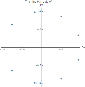
Here, for example, are nine 9th roots of -1:

In[1]:= rootOfMinusOne[k_, n_] := Exp[(2 k + 1) Pi I/n]

In[2]:= roots9 = Table[rootOfMinusOne[k, 9], {k, 9}]

Out[2]= {E^((I \[Pi])/3), E^((5 I \[Pi])/9), E^((
 7 I \[Pi])/9), -1, E^(-((7 I \[Pi])/9)), E^(-((5 I \[Pi])/9)), E^(-((
  I \[Pi])/3)), E^(-((I \[Pi])/9)), E^((I \[Pi])/9)}

In[3]:= #^9 & /@ roots9

Out[3]= {-1, -1, -1, -1, -1, -1, -1, -1, -1}

In[4]:= cPlot[lst_, opts___] := 
 ListPlot[{Re[#], Im[#]} & /@ lst, AspectRatio -> 1, 
  AxesLabel -> {"Re", "Im"}, opts]

In[5]:= cplt = cPlot[roots9, PlotLabel -> "The nine 9th roots of -1"]

enter image description here

POSTED BY: David Keith
Posted 9 years ago

Thank you, David. I must give credit where credit is due, to Leonhard Euler!

I was wondering whether someone might suggest a parametric plot for representing real and imaginary components. It is Pi Day after all! An alternate, continuous representation that includes the subset you've explored above:

ParametricPlot[{Cos[u], Sin[u]}, {u, 0, 2 Pi}, 
 PlotLabel -> "Cos \[Phi] + \[ImaginaryI] Sin \[Phi]", 
 AxesLabel -> {"Re", "Im"}]

unit<em>circleparametric_plot

POSTED BY: Caitlin Ramsey
Posted 9 years ago

If we have to cite Euler every time we use his discoveries we will all spend half our time writing citations. ;-)

Happy Pi Day!

enter image description here

POSTED BY: David Keith

Do you have examples available? Without that it's impossible to tell if you are running into numerical issues or getting legitimate but surprising results.

POSTED BY: Daniel Lichtblau
Posted 9 years ago

You sound like a lawyer: it depends! LOL

Is there a way of either eliminating the component or deciding that it can be ignored? Is this even the correct question?

In responding to Daniel Lichtblau's requests, I discovered that I have eliminated this issue by my choice of doing NIntegrate and avoiding Integrate. I cannot find the worksheet that was giving me the imaginary results.

I may have wasted the group's time on this topic, despite what I have learned, since the issue now is whether my NIntegrate and NumericQ parametric plots are leading me astray.

POSTED BY: Luther Nayhm

I'm a physicist. I'm used to mathematics needing guidance to properly represent physical reality. It starts with very simple high school problems. Consider dropping a ball: how long will it take to hit the floor. Well, it's the solution to an algebra problem:

In[24]:= Solve[ 1/2 a t^2 == h, t]

Out[24]= {{t -> -((Sqrt[2] Sqrt[h])/Sqrt[a])}, {t -> (
   Sqrt[2] Sqrt[h])/Sqrt[a]}}

Oops, there are two solutions! However, the ball can't hit the floor before you drop it, so we throw out the negative one. This is completely normal.

Now, for algebra problems there are "root isolation" methods that find all solutions rigorously, and Mathematica uses them. So, you throw out the solutions you don't want and you have the solutions for your problem. However, once you go beyond algebra, you generally can't have confidence that your method, even if it has found a solution, has found every solution to your mathematical problem, nor can you be certain that the solution it has found is the solution that you want for your physical problem. You're in the realm of "experimental verification".

Comparing results from Integrate and NIntegrate is a good sort of mathematical experiment, as they have different sorts of problems. You've already encountered Integrate's branch cut trouble. NIntegrate has the problem that if its sampling of points in the function in question accidentally misses the exciting parts, it may yield an entirely bogus result.

Mathematica will not do your thinking for you.

POSTED BY: John Doty
Posted 9 years ago

Hello guys, can you help me with my problem in this thread?

http://community.wolfram.com/groups/-/m/t/455321

in that discussion, the formula is just an example of my work using ParametricNDSolveValue, the problem surfaced when FindRoot have an answer of complex value. is there anyway to force FindRoot to present only Real numbers?

POSTED BY: Thai Kee Gan

This discussion (thread) was locked.

It is getting too many follow-up questions that deserve their own discussions.

Moderation Staff

POSTED BY: Moderation Team

Group Abstract Group Abstract