Message Boards Message Boards

0
|
35421 Views
|
20 Replies
|
8 Total Likes
View groups...
Share
Share this post:

How to plot the graph of the equation F[x,y]=0 ?

Posted 10 years ago

I have an equation F(x,y;a,b,c,...)=0, where x and y are variables, a,b,c,... - parameters. y is a real number, x - complex. For every given y I need to solve this equation, i.e. to find Im(x) and Re(x) (this equation may have many solutions). After solving this equation I need to plot two graphs: the dependense of y from Im(x) and y from Re(x).

For example, F(x,y)=x^2 + sin(xy).

If y and x were real numbers, it would be possible to use ContourPlot. However, as my variables are complex, I have to solve this equation numerically and after that plot my graphs.

I have never come across such a problem (and also to date I have a little experience in Mathematica), so could anyone tell me how to solve this problem?

POSTED BY: Artem Strashko
20 Replies

You might do better to define a root-finding function that, given a value for y, finds Re[x] and Im[x]. Using the redefined form I showed earlier, with s and t as variables for the real and imaginary parts of x respectively, this might be done as below. I use random starting points so as to have a chance at sampling from different branches of the solution curve.

root[yval_?NumericQ] := {s, t} /. 
  FindRoot[{re == 0, im == 0} /. y -> yval, {s, 
    RandomReal[{-5, 5}]}, {t, RandomReal[{-5, 5}]}]

Here is how it looks.

pts = Quiet[Table[root[j], {j, .01, 8, .01}]];
ListPlot[pts]

enter image description here

POSTED BY: Daniel Lichtblau

This might be a start. Define the expression, then use ComplexExpand to form explicit real and imaginary parts.

g = 1/10;
expr = 
  Tanh[Sqrt[-x^2 - y^2]*3/10] (y^2 + I*g*y - 4) Sqrt[-x^2 - 
      y^2] + (y^2 + I*g*y) Sqrt[-x^2 - 
      y^2 ((y^2 + I*g*y - 4)/(y^2 + I*g*y))];

e2 = expr /. x -> s + I*t;
{re, im} = ComplexExpand[{Re[e2], Im[e2]}];

 ContourPlot[(re /. y -> 0.7) == 0, {s, -10, 10}, {t, -10, 10}]

enter image description here

ContourPlot[(im /. y -> 0.7) == 0, {s, -10, 10}, {t, -10, 10}]

enter image description here

POSTED BY: Daniel Lichtblau

You will get better answers if you give a complete, very specific example of what you want.

POSTED BY: Daniel Lichtblau

Use ContourPlot3D, it should give you your result; a 3d surface.

POSTED BY: Sander Huisman
Posted 10 years ago

Dear Sander, I try to use ContourPlot3D for a very simple problem, but it doesn't give a right answer.enter image description here

Attachments:
POSTED BY: Artem Strashko
Posted 10 years ago
POSTED BY: Artem Strashko
Posted 10 years ago

Dear Daniel, thank you so much for your help! Hovewer, I am not sure that this is exactly what I need, because I don't quietly understand how it works.

I can explain what I need in other words. I need the graph of the equation F[x,y]=0, x is a complex number, y is a real number, {y,0,8}. The graph of this equation is 3D, because we have 3 variables Re[x], Im[x], y. I need two 2D graphs y as a function of Re[x] and Im[x], I mean that I need two projection of this 3D graph.I mean smth like that

POSTED BY: Artem Strashko
Posted 10 years ago

Thank you. But can I further extract two 2D graphs from this 3D graph? I mean I can plot F[Re[x],Im[x],y]=0, but I would like to get two projections of this graph: Re[x],y and Im[x],y.

POSTED BY: Artem Strashko
Posted 10 years ago

Dear Daniel, could you clarify how do you do this? I try to use your code, but I don't get a result.g = 1/10; expr = x - Sqrt[y^2 + I*y]; e2 = expr /. x -> s + I*t; {re, im} = ComplexExpand[{Re[e2], Im[e2]}]; root[yval_?NumericQ] := {s, t} /. FindRoot[{re == 0, im == 0} /. y -> yval, {s, RandomReal[{-5, 5}]}, {t, RandomReal[{-5, 5}]}] pts = Quiet[Table[root[j], {j, .01, 8, .01}]]; ListPlot[pts]

Attachments:
POSTED BY: Artem Strashko

Your nb gave a nice plot when I executed the top cell. Maybe you had other definitions active at the time that interfered in some way?

POSTED BY: Daniel Lichtblau
Posted 10 years ago

Dear Daniel, I am sorry for interruption. I don't know what was the problem, but now everything is fine. Could you answer a couple of other questions? Firstly, what shoul I do to consider this problem only in the region {Im[x],0,8}, {Re[x],0,8}, {y,0,8}. And how can I distinguish between the dependense of y on Re[x] and y on Im[x] depicted on the figure? Also, could you clarify what do I change when alter RandomReal[{0, 5}] and {j, .01, 5, .01}?

Attachments:
POSTED BY: Artem Strashko
Posted 10 years ago

Dear Daniel. I have decided to check your method I have considered a very simple problem (x=f[y]) which can be easily solved by a very straightforward method (just using Plot). I don't know why but the results are essentially different.

I attach my file, but the general idea is very simple. If we have x = f[y] and x=x'+ix'', we can just plot x'=Re[f[y]] and x''=Im[f[y]] and compare these graphs with the graphs which we get using your method.

Attachments:
POSTED BY: Artem Strashko

The plots look more similar if you recognize that the equivalent form for the second one should use ParametricPlot instead of Plot (such distinctions are very important). The ListPlot will need a range setting as well. Try the two below.

ListPlot[pts, PlotRange -> All]

ParametricPlot[{Re[y*Sqrt[(y^2 + 1/10*I*y - 4)/(2 y^2 + 1/10*2*I*y - 4)]], 
  Im[y*Sqrt[(y^2 + 1/10*I*y - 4)/(2 y^2 + 1/10*2*I*y - 4)]]}, {y,  0.0001, 4}, PlotRange -> All]
POSTED BY: Daniel Lichtblau
Posted 10 years ago
Attachments:
POSTED BY: Artem Strashko

I was simply explaining why the plots were different.

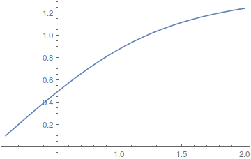
As for getting y as functions, respectively, of Re[x] and Im[x], that gets tricky because it is in general not a function but rather a "multivalued function". You will probably want to get a continuous branch of such inverses. One method you might consider is to find a value for y at a given re(x), say, and then trace from there by setting up an NDSolve equation.

Lets define the real and imaginary parts of f as ref and imf respectively. And the real and imaginary parts of x we will call rex and imx. The equations you have are {ref[rex,imx,y]==0,imf[rex,imx,y]==0}. To inverst y in terms of rex, treat it as a function of rex (the whole point of the exercise) and differentiate. I'll show explicit code for your example.

expr = y*Sqrt[(y^2 + 1/10*I*y - 4)/(2 y^2 + 1/10*2*I*y - 4)];
sys = {rex, imx} - ComplexExpand[{Re[expr], Im[expr]},TargetFunctions -> {Re, Im}];
dsys = D[sys /. {y -> y[rex], imx -> imx[rex]}, rex];
yinit = .1;
init = expr /. y -> yinit;

soly = NDSolveValue[Flatten[{Thread[dsys == 0], y[Re[init]] == yinit, 
    imx[Re[init]] == Im[init]}], y[rex], {rex, Re[init], 2}]

(* Out[77]= InterpolatingFunction[{{0.100125, 2.}}, <>][rex] *)

Plot[soly, {rex, Re[init], 2}]
enter image description here

POSTED BY: Daniel Lichtblau
Posted 10 years ago

Dear Daniel, thank you for you help. Could you tell me what version of Mathematica do you use (because I can't use this code in my version 7)?

POSTED BY: Artem Strashko

I'm using version 10.1. You can do similarly with NDSolve if you solve for both {y[rex],imx[rex]}.

POSTED BY: Daniel Lichtblau
Posted 10 years ago

Ok, thanks!

POSTED BY: Artem Strashko
Posted 10 years ago

Dear Daniel, I have installed Mathematica 10, but again I can't use your code.

Attachments:
POSTED BY: Artem Strashko

You should do some debugging. Look hard at the messages, the NDSolveValue result, that sort of thing. Maybe even start in a fresh kernel.

POSTED BY: Daniel Lichtblau
Reply to this discussion
Community posts can be styled and formatted using the Markdown syntax.
Reply Preview
Attachments
Remove
or Discard

Group Abstract Group Abstract