Group Abstract Group Abstract

Message Boards Message Boards

0
|
8.7K Views
|
12 Replies
|
9 Total Likes
View groups...
Share
Share this post:

Need help with "FindFit"

Posted 11 years ago

Hello, I'm trying to fit a gaussian curve to a data table, but I get an error message I dont understand.

FindFit[%1, a exp[(-b + x)^2/c], {{a, 700}, {b, 3490}, {c, 20}}, x]

FindFit::nrlnum: The function value {-16.+700. exp[400.513],-32.+700. exp[391.613],-24.+700. exp[382.813],-28.+700. exp[374.113],-21.+700. exp[365.513],-25.+700. exp[357.013],<<39>>,-191.+700. exp[99.0125],-185.+700. exp[94.6125],-189.+700. exp[90.3125],-208.+700. exp[86.1125],-227.+700. exp[82.0125],<<71>>} is not a list of real numbers with dimensions {121} at {a,b,c} = {700.,3490.,20.}. >>

The data input is:

{{3400.5, 16}, {3401.5, 32}, {3402.5, 24}, {3403.5, 28}, {3404.5, 21}, {3405.5, 25}, {3406.5, 24}, {3407.5, 28}, {3408.5, 34}, {3409.5, 28}, {3410.5, 26}, {3411.5, 38}, {3412.5, 26}, {3413.5, 30}, {3414.5, 41}, {3415.5, 44}, {3416.5, 30}, {3417.5, 34}, {3418.5, 50}, {3419.5, 55}, {3420.5, 48}, {3421.5, 60}, {3422.5, 66}, {3423.5, 59}, {3424.5, 81}, {3425.5, 73}, {3426.5, 77}, {3427.5, 61}, {3428.5, 89}, {3429.5, 92}, {3430.5, 74}, {3431.5, 97}, {3432.5, 99}, {3433.5, 107}, {3434.5, 104}, {3435.5, 104}, {3436.5, 107}, {3437.5, 140}, {3438.5, 129}, {3439.5, 120}, {3440.5, 143}, {3441.5, 158}, {3442.5, 148}, {3443.5, 143}, {3444.5, 184}, {3445.5, 191}, {3446.5, 185}, {3447.5, 189}, {3448.5, 208}, {3449.5, 227}, {3450.5, 231}, {3451.5, 244}, {3452.5, 261}, {3453.5, 268}, {3454.5, 302}, {3455.5, 306}, {3456.5, 332}, {3457.5, 337}, {3458.5, 357}, {3459.5, 347}, {3460.5, 347}, {3461.5, 401}, {3462.5, 396}, {3463.5, 432}, {3464.5, 422}, {3465.5, 428}, {3466.5, 469}, {3467.5, 472}, {3468.5, 451}, {3469.5, 456}, {3470.5, 449}, {3471.5, 477}, {3472.5, 509}, {3473.5, 513}, {3474.5, 482}, {3475.5, 480}, {3476.5, 500}, {3477.5, 508}, {3478.5, 522}, {3479.5, 519}, {3480.5, 550}, {3481.5, 576}, {3482.5, 590}, {3483.5, 628}, {3484.5, 646}, {3485.5, 709}, {3486.5, 700}, {3487.5, 706}, {3488.5, 732}, {3489.5, 683}, {3490.5, 732}, {3491.5, 711}, {3492.5, 697}, {3493.5, 603}, {3494.5, 657}, {3495.5, 571}, {3496.5, 526}, {3497.5, 470}, {3498.5, 427}, {3499.5, 358}, {3500.5, 339}, {3501.5, 307}, {3502.5, 251}, {3503.5, 201}, {3504.5, 147}, {3505.5, 139}, {3506.5, 122}, {3507.5, 95}, {3508.5, 51}, {3509.5, 66}, {3510.5, 39}, {3511.5, 37}, {3512.5, 29}, {3513.5, 18}, {3514.5, 19}, {3515.5, 13}, {3516.5, 5}, {3517.5, 4}, {3518.5, 8}, {3519.5, 8}, {3520.5`, 1}}

I would appreciate your help =)

POSTED BY: Florian Graf
12 Replies
Posted 11 years ago

And thinking a little more, this looked suspiciously like a superposition of Gaussians. Does theory justify such an interpretation?

In[31]:= fit2 = 
  NonlinearModelFit[data, 
   a Exp[-(-b + x)^2/c] + 
    a1 Exp[-(-b1 + x)^2/c1], {{a, 700}, {b, 3490}, {c, 20}, {a1, 
     700}, {b1, 3490}, {c1, 20}}, x];

In[32]:= fit2["BestFitParameters"]

Out[32]= {a -> 456.927, b -> 3490.81, c -> 106.369, a1 -> 441.68, 
 b1 -> 3470.54, c1 -> 766.738}

In[33]:= Show[Plot[fit2[x], {x, 3400, 3520}, PlotStyle -> Red], 
 ListPlot@data, PlotRange -> All]

enter image description here

POSTED BY: David Keith

To reiterate what ^Jim Baldwin said, are you sure you don't want to use FindDistributionParameters?

Using NonlinearModelFit to estimate the parameters of a distribution is a very common mistake.

POSTED BY: Sean Clarke
Posted 11 years ago

The exponent of the Gaussian needs to be negative. I used NonlinearModelFit below, but FindFit would work.

In[25]:= fit = 
  NonlinearModelFit[data, 
   a Exp[-(-b + x)^2/c], {{a, 700}, {b, 3490}, {c, 20}}, x];

In[26]:= fit["BestFitParameters"]

Out[26]= {a -> 622.26, b -> 3479.8, c -> 728.5}

In[27]:= Show[Plot[fit[x], {x, 3400, 3520}, PlotStyle -> Red], 
 ListPlot@data, PlotRange -> All]

enter image description here

POSTED BY: David Keith
Posted 11 years ago

To follow on David Keith's question: What is the process that generates these points?

I see that the points on the horizontal axis are equally-spaced with a unit of 1 between each point. The vertical axis variable values are all integers and if those integers are counts, then they appear to be a bit under-dispersed for Poisson counts.

I ask these questions in part to attempt to ascertain what the expected variance structure of the residuals might be. For example, is serial correlation expected? Also, do you just need a "good fit" as opposed to needing to estimate coefficients from some theoretical model?

POSTED BY: Jim Baldwin
Posted 11 years ago

You need "Exp" rather than "exp". (But the plot of the data suggests that a such a curve will not be a very good fit.)

POSTED BY: Jim Baldwin
Posted 11 years ago

If the data represent histogram information, then the raw data (if available) could be used to construct a nonparametric density estimate if a good description of the shape is adequate (as opposed to a need to interpret parameters in say a more parametric mixture distribution). Alternatively because there is so much data the raw data can be approximated by using the histogram bin values and the frequency counts:

(* Histogram information *)
data = {{3400.5, 16}, {3401.5, 32}, {3402.5, 24}, {3403.5, 
    28}, {3404.5, 21}, {3405.5, 25}, {3406.5, 24}, {3407.5, 
    28}, {3408.5, 34}, {3409.5, 28}, {3410.5, 26}, {3411.5, 
    38}, {3412.5, 26}, {3413.5, 30}, {3414.5, 41}, {3415.5, 
    44}, {3416.5, 30}, {3417.5, 34}, {3418.5, 50}, {3419.5, 
    55}, {3420.5, 48}, {3421.5, 60}, {3422.5, 66}, {3423.5, 
    59}, {3424.5, 81}, {3425.5, 73}, {3426.5, 77}, {3427.5, 
    61}, {3428.5, 89}, {3429.5, 92}, {3430.5, 74}, {3431.5, 
    97}, {3432.5, 99}, {3433.5, 107}, {3434.5, 104}, {3435.5, 
    104}, {3436.5, 107}, {3437.5, 140}, {3438.5, 129}, {3439.5, 
    120}, {3440.5, 143}, {3441.5, 158}, {3442.5, 148}, {3443.5, 
    143}, {3444.5, 184}, {3445.5, 191}, {3446.5, 185}, {3447.5, 
    189}, {3448.5, 208}, {3449.5, 227}, {3450.5, 231}, {3451.5, 
    244}, {3452.5, 261}, {3453.5, 268}, {3454.5, 302}, {3455.5, 
    306}, {3456.5, 332}, {3457.5, 337}, {3458.5, 357}, {3459.5, 
    347}, {3460.5, 347}, {3461.5, 401}, {3462.5, 396}, {3463.5, 
    432}, {3464.5, 422}, {3465.5, 428}, {3466.5, 469}, {3467.5, 
    472}, {3468.5, 451}, {3469.5, 456}, {3470.5, 449}, {3471.5, 
    477}, {3472.5, 509}, {3473.5, 513}, {3474.5, 482}, {3475.5, 
    480}, {3476.5, 500}, {3477.5, 508}, {3478.5, 522}, {3479.5, 
    519}, {3480.5, 550}, {3481.5, 576}, {3482.5, 590}, {3483.5, 
    628}, {3484.5, 646}, {3485.5, 709}, {3486.5, 700}, {3487.5, 
    706}, {3488.5, 732}, {3489.5, 683}, {3490.5, 732}, {3491.5, 
    711}, {3492.5, 697}, {3493.5, 603}, {3494.5, 657}, {3495.5, 
    571}, {3496.5, 526}, {3497.5, 470}, {3498.5, 427}, {3499.5, 
    358}, {3500.5, 339}, {3501.5, 307}, {3502.5, 251}, {3503.5, 
    201}, {3504.5, 147}, {3505.5, 139}, {3506.5, 122}, {3507.5, 
    95}, {3508.5, 51}, {3509.5, 66}, {3510.5, 39}, {3511.5, 
    37}, {3512.5, 29}, {3513.5, 18}, {3514.5, 19}, {3515.5, 
    13}, {3516.5, 5}, {3517.5, 4}, {3518.5, 8}, {3519.5, 8}, {3520.5, 
    1}};

(* "Reconstruct" raw data *)
rawData = Table[0, {i, Total[data[[All, 2]]]}];
n = 0;
Do[Do[n = n + 1; rawData[[n]] = data[[i, 1]], {j, data[[i, 2]]}], {i, 
  Length[data[[All, 1]]]}]

(* Construct nonparametric density estimate *)
f = SmoothKernelDistribution[rawData];

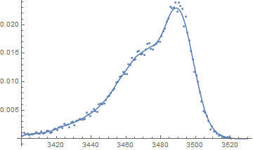
(* Plot relative frequencies and nonparametric density estimate *)
Show[{
  Plot[PDF[f, x], {x, 3400, 3530}],
  ListPlot[
   Table[{data[[i, 1]], data[[i, 2]]/n}, {i, Length[data[[All, 1]]]}]]
  }]

Nonparametric density estimate

POSTED BY: Jim Baldwin
Posted 11 years ago

Thanks, Marco -- I was not thinking at all clearly about this problem. We are given a PDF -- to fit a distribution we have to reconstitute the samples themselves, as you did with data2. Following you, I tiried to fit this to a superposition of normal distributions, with the same result.

In[241]:= candidate2 = 
 MixtureDistribution[{a1, a2}, {NormalDistribution[u1, s1], 
   NormalDistribution[u2, s2]}]

Out[241]= MixtureDistribution[{a1, a2}, {NormalDistribution[u1, s1], 
  NormalDistribution[u2, s2]}]

In[242]:= par2 = FindDistributionParameters[
  data2,
  candidate2,
  {{a1, 1000}, {a2, 1000}, {u1, 3460}, {s1, 10}, {u2, 3490}, {s2, 10}}]

During evaluation of In[242]:= FindMaximum::eit: The algorithm does not converge to the tolerance of 4.806217383937354`*^-6 in 500 iterations. The best estimated solution, with feasibility residual, KKT residual, or complementary residual of {1.83244*10^-9,0.00273008,4.85286*10^-10}, is returned. >>

Out[242]= {a1 -> 1187.93, a2 -> 866.089, u1 -> 3462.92, s1 -> 21.0563,
  u2 -> 3488.61, s2 -> 9.17502}

In[243]:= dist = candidate2 /. par2;

In[244]:= Show[
 Plot[Length[data2] PDF[dist][x], {x, 3400, 3520}, PlotStyle -> Red], 
 ListPlot@data, PlotRange -> All]

enter image description here

POSTED BY: David Keith

Hi,

the following "solution" uses the new and experimental function FindDistribution. The results are not perfect, but anyway.

data2 = Flatten[Table[#[[1]], {k, 1, #[[2]]}] & /@ data];
dist = FindDistribution[data2, MaxItems -> 3, TargetFunctions -> All, PerformanceGoal -> "Quality"];
(*MixtureDistribution[{0.545163, 0.454837}, {NormalDistribution[3461.87, 20.9496], NormalDistribution[3488.13, 9.61732]}]*)
Show[Histogram[data2, 400, "Probability"], Plot[PDF[dist, x], {x, 3400, 3520}, PlotRange -> All]]

enter image description here

You can also ask for a list of most likely distributions:

dist = FindDistribution[data2, 3, PerformanceGoal -> "Quality"]
(*{MixtureDistribution[{0.545163, 0.454837}, {NormalDistribution[3461.87, 20.9496], NormalDistribution[3488.13, 9.61732]}], 
 WeibullDistribution[198.987, 3483.87], 
 GumbelDistribution[3483.91, 17.4908]}*)

Cheers,

Marco

POSTED BY: Marco Thiel
Posted 11 years ago

While FindDistributionParameters might provide a reasonable "fit" that well describes the observed data (a mixture of two or more normals for example), there is no random sampling from a mixture of normal distributions or a mixture of Poisson distributions. The counts likely have a random component (approximately Poisson) but not the particle energy variable (as those values are uniformly spaced and not randomly distributed).

It appears that what you have is a Poisson regression with the particle's energy as the fixed and known predictor and the counts as the dependent variable. As the plot of the data shows, this is not a simple linear or quadratic relationship. I think what you need is a generalized additive model (gam) but I'm unaware of a Mathematica-supplied function for that. However, you could call the appropriate function in R from Mathematica using R's mgcv library.

An update: I'll backtrack a bit (well, a whole lot) if the equal-spaced energy values and the counts represent a histogram with the particle energy values parked in the appropriate bins. Then you are in the mode of fitting a distribution rather than a Poisson regression. But if the particle energy levels are specifically set and increased from the lowest value to the highest, then a Poisson regression is more appropriate.

POSTED BY: Jim Baldwin
Posted 11 years ago

Quite interesting. Perhaps some more discussion??

In[107]:= candidate1 = 
 MixtureDistribution[{a1, a2}, {PoissonDistribution[u1], 
   PoissonDistribution[u2]}]

Out[107]= MixtureDistribution[{a1, a2}, {PoissonDistribution[u1], 
  PoissonDistribution[u2]}]

In[108]:= FindDistributionParameters[
 data,
 candidate,
 {{a1, 100000}, {a2, 100000}, {u1, 3460}, {u2, 3490}}]

During evaluation of In[108]:= FindDistributionParameters::ntsprt: One or more data points are not in support of the process or distribution MixtureDistribution[{a1,a2},{PoissonDistribution[u1],PoissonDistribution[u2]}]. >>
POSTED BY: David Keith
Posted 11 years ago
POSTED BY: Florian Graf
Posted 11 years ago

Wow, didnt think that it would be so easy :D

what kind of curve would you suggest?

POSTED BY: Florian Graf
Reply to this discussion
Community posts can be styled and formatted using the Markdown syntax.
Reply Preview
Attachments
Remove
or Discard