Message Boards Message Boards

0
|
7830 Views
|
12 Replies
|
9 Total Likes
View groups...
Share
Share this post:

Need help with "FindFit"

Posted 10 years ago

Hello, I'm trying to fit a gaussian curve to a data table, but I get an error message I dont understand.

FindFit[%1, a exp[(-b + x)^2/c], {{a, 700}, {b, 3490}, {c, 20}}, x]

FindFit::nrlnum: The function value {-16.+700. exp[400.513],-32.+700. exp[391.613],-24.+700. exp[382.813],-28.+700. exp[374.113],-21.+700. exp[365.513],-25.+700. exp[357.013],<<39>>,-191.+700. exp[99.0125],-185.+700. exp[94.6125],-189.+700. exp[90.3125],-208.+700. exp[86.1125],-227.+700. exp[82.0125],<<71>>} is not a list of real numbers with dimensions {121} at {a,b,c} = {700.,3490.,20.}. >>

The data input is:

{{3400.5, 16}, {3401.5, 32}, {3402.5, 24}, {3403.5, 28}, {3404.5, 21}, {3405.5, 25}, {3406.5, 24}, {3407.5, 28}, {3408.5, 34}, {3409.5, 28}, {3410.5, 26}, {3411.5, 38}, {3412.5, 26}, {3413.5, 30}, {3414.5, 41}, {3415.5, 44}, {3416.5, 30}, {3417.5, 34}, {3418.5, 50}, {3419.5, 55}, {3420.5, 48}, {3421.5, 60}, {3422.5, 66}, {3423.5, 59}, {3424.5, 81}, {3425.5, 73}, {3426.5, 77}, {3427.5, 61}, {3428.5, 89}, {3429.5, 92}, {3430.5, 74}, {3431.5, 97}, {3432.5, 99}, {3433.5, 107}, {3434.5, 104}, {3435.5, 104}, {3436.5, 107}, {3437.5, 140}, {3438.5, 129}, {3439.5, 120}, {3440.5, 143}, {3441.5, 158}, {3442.5, 148}, {3443.5, 143}, {3444.5, 184}, {3445.5, 191}, {3446.5, 185}, {3447.5, 189}, {3448.5, 208}, {3449.5, 227}, {3450.5, 231}, {3451.5, 244}, {3452.5, 261}, {3453.5, 268}, {3454.5, 302}, {3455.5, 306}, {3456.5, 332}, {3457.5, 337}, {3458.5, 357}, {3459.5, 347}, {3460.5, 347}, {3461.5, 401}, {3462.5, 396}, {3463.5, 432}, {3464.5, 422}, {3465.5, 428}, {3466.5, 469}, {3467.5, 472}, {3468.5, 451}, {3469.5, 456}, {3470.5, 449}, {3471.5, 477}, {3472.5, 509}, {3473.5, 513}, {3474.5, 482}, {3475.5, 480}, {3476.5, 500}, {3477.5, 508}, {3478.5, 522}, {3479.5, 519}, {3480.5, 550}, {3481.5, 576}, {3482.5, 590}, {3483.5, 628}, {3484.5, 646}, {3485.5, 709}, {3486.5, 700}, {3487.5, 706}, {3488.5, 732}, {3489.5, 683}, {3490.5, 732}, {3491.5, 711}, {3492.5, 697}, {3493.5, 603}, {3494.5, 657}, {3495.5, 571}, {3496.5, 526}, {3497.5, 470}, {3498.5, 427}, {3499.5, 358}, {3500.5, 339}, {3501.5, 307}, {3502.5, 251}, {3503.5, 201}, {3504.5, 147}, {3505.5, 139}, {3506.5, 122}, {3507.5, 95}, {3508.5, 51}, {3509.5, 66}, {3510.5, 39}, {3511.5, 37}, {3512.5, 29}, {3513.5, 18}, {3514.5, 19}, {3515.5, 13}, {3516.5, 5}, {3517.5, 4}, {3518.5, 8}, {3519.5, 8}, {3520.5`, 1}}

I would appreciate your help =)

POSTED BY: Florian Graf
12 Replies
Posted 10 years ago

If the data represent histogram information, then the raw data (if available) could be used to construct a nonparametric density estimate if a good description of the shape is adequate (as opposed to a need to interpret parameters in say a more parametric mixture distribution). Alternatively because there is so much data the raw data can be approximated by using the histogram bin values and the frequency counts:

(* Histogram information *)
data = {{3400.5, 16}, {3401.5, 32}, {3402.5, 24}, {3403.5, 
    28}, {3404.5, 21}, {3405.5, 25}, {3406.5, 24}, {3407.5, 
    28}, {3408.5, 34}, {3409.5, 28}, {3410.5, 26}, {3411.5, 
    38}, {3412.5, 26}, {3413.5, 30}, {3414.5, 41}, {3415.5, 
    44}, {3416.5, 30}, {3417.5, 34}, {3418.5, 50}, {3419.5, 
    55}, {3420.5, 48}, {3421.5, 60}, {3422.5, 66}, {3423.5, 
    59}, {3424.5, 81}, {3425.5, 73}, {3426.5, 77}, {3427.5, 
    61}, {3428.5, 89}, {3429.5, 92}, {3430.5, 74}, {3431.5, 
    97}, {3432.5, 99}, {3433.5, 107}, {3434.5, 104}, {3435.5, 
    104}, {3436.5, 107}, {3437.5, 140}, {3438.5, 129}, {3439.5, 
    120}, {3440.5, 143}, {3441.5, 158}, {3442.5, 148}, {3443.5, 
    143}, {3444.5, 184}, {3445.5, 191}, {3446.5, 185}, {3447.5, 
    189}, {3448.5, 208}, {3449.5, 227}, {3450.5, 231}, {3451.5, 
    244}, {3452.5, 261}, {3453.5, 268}, {3454.5, 302}, {3455.5, 
    306}, {3456.5, 332}, {3457.5, 337}, {3458.5, 357}, {3459.5, 
    347}, {3460.5, 347}, {3461.5, 401}, {3462.5, 396}, {3463.5, 
    432}, {3464.5, 422}, {3465.5, 428}, {3466.5, 469}, {3467.5, 
    472}, {3468.5, 451}, {3469.5, 456}, {3470.5, 449}, {3471.5, 
    477}, {3472.5, 509}, {3473.5, 513}, {3474.5, 482}, {3475.5, 
    480}, {3476.5, 500}, {3477.5, 508}, {3478.5, 522}, {3479.5, 
    519}, {3480.5, 550}, {3481.5, 576}, {3482.5, 590}, {3483.5, 
    628}, {3484.5, 646}, {3485.5, 709}, {3486.5, 700}, {3487.5, 
    706}, {3488.5, 732}, {3489.5, 683}, {3490.5, 732}, {3491.5, 
    711}, {3492.5, 697}, {3493.5, 603}, {3494.5, 657}, {3495.5, 
    571}, {3496.5, 526}, {3497.5, 470}, {3498.5, 427}, {3499.5, 
    358}, {3500.5, 339}, {3501.5, 307}, {3502.5, 251}, {3503.5, 
    201}, {3504.5, 147}, {3505.5, 139}, {3506.5, 122}, {3507.5, 
    95}, {3508.5, 51}, {3509.5, 66}, {3510.5, 39}, {3511.5, 
    37}, {3512.5, 29}, {3513.5, 18}, {3514.5, 19}, {3515.5, 
    13}, {3516.5, 5}, {3517.5, 4}, {3518.5, 8}, {3519.5, 8}, {3520.5, 
    1}};

(* "Reconstruct" raw data *)
rawData = Table[0, {i, Total[data[[All, 2]]]}];
n = 0;
Do[Do[n = n + 1; rawData[[n]] = data[[i, 1]], {j, data[[i, 2]]}], {i, 
  Length[data[[All, 1]]]}]

(* Construct nonparametric density estimate *)
f = SmoothKernelDistribution[rawData];

(* Plot relative frequencies and nonparametric density estimate *)
Show[{
  Plot[PDF[f, x], {x, 3400, 3530}],
  ListPlot[
   Table[{data[[i, 1]], data[[i, 2]]/n}, {i, Length[data[[All, 1]]]}]]
  }]
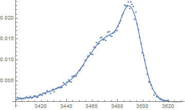
Nonparametric density estimate

POSTED BY: Jim Baldwin
Posted 10 years ago

Thanks, Marco -- I was not thinking at all clearly about this problem. We are given a PDF -- to fit a distribution we have to reconstitute the samples themselves, as you did with data2. Following you, I tiried to fit this to a superposition of normal distributions, with the same result.

In[241]:= candidate2 = 
 MixtureDistribution[{a1, a2}, {NormalDistribution[u1, s1], 
   NormalDistribution[u2, s2]}]

Out[241]= MixtureDistribution[{a1, a2}, {NormalDistribution[u1, s1], 
  NormalDistribution[u2, s2]}]

In[242]:= par2 = FindDistributionParameters[
  data2,
  candidate2,
  {{a1, 1000}, {a2, 1000}, {u1, 3460}, {s1, 10}, {u2, 3490}, {s2, 10}}]

During evaluation of In[242]:= FindMaximum::eit: The algorithm does not converge to the tolerance of 4.806217383937354`*^-6 in 500 iterations. The best estimated solution, with feasibility residual, KKT residual, or complementary residual of {1.83244*10^-9,0.00273008,4.85286*10^-10}, is returned. >>

Out[242]= {a1 -> 1187.93, a2 -> 866.089, u1 -> 3462.92, s1 -> 21.0563,
  u2 -> 3488.61, s2 -> 9.17502}

In[243]:= dist = candidate2 /. par2;

In[244]:= Show[
 Plot[Length[data2] PDF[dist][x], {x, 3400, 3520}, PlotStyle -> Red], 
 ListPlot@data, PlotRange -> All]

enter image description here

POSTED BY: David Keith

Hi,

the following "solution" uses the new and experimental function FindDistribution. The results are not perfect, but anyway.

data2 = Flatten[Table[#[[1]], {k, 1, #[[2]]}] & /@ data];
dist = FindDistribution[data2, MaxItems -> 3, TargetFunctions -> All, PerformanceGoal -> "Quality"];
(*MixtureDistribution[{0.545163, 0.454837}, {NormalDistribution[3461.87, 20.9496], NormalDistribution[3488.13, 9.61732]}]*)
Show[Histogram[data2, 400, "Probability"], Plot[PDF[dist, x], {x, 3400, 3520}, PlotRange -> All]]

enter image description here

You can also ask for a list of most likely distributions:

dist = FindDistribution[data2, 3, PerformanceGoal -> "Quality"]
(*{MixtureDistribution[{0.545163, 0.454837}, {NormalDistribution[3461.87, 20.9496], NormalDistribution[3488.13, 9.61732]}], 
 WeibullDistribution[198.987, 3483.87], 
 GumbelDistribution[3483.91, 17.4908]}*)

Cheers,

Marco

POSTED BY: Marco Thiel
Posted 10 years ago

While FindDistributionParameters might provide a reasonable "fit" that well describes the observed data (a mixture of two or more normals for example), there is no random sampling from a mixture of normal distributions or a mixture of Poisson distributions. The counts likely have a random component (approximately Poisson) but not the particle energy variable (as those values are uniformly spaced and not randomly distributed).

It appears that what you have is a Poisson regression with the particle's energy as the fixed and known predictor and the counts as the dependent variable. As the plot of the data shows, this is not a simple linear or quadratic relationship. I think what you need is a generalized additive model (gam) but I'm unaware of a Mathematica-supplied function for that. However, you could call the appropriate function in R from Mathematica using R's mgcv library.

An update: I'll backtrack a bit (well, a whole lot) if the equal-spaced energy values and the counts represent a histogram with the particle energy values parked in the appropriate bins. Then you are in the mode of fitting a distribution rather than a Poisson regression. But if the particle energy levels are specifically set and increased from the lowest value to the highest, then a Poisson regression is more appropriate.

POSTED BY: Jim Baldwin
Posted 10 years ago

Quite interesting. Perhaps some more discussion??

In[107]:= candidate1 = 
 MixtureDistribution[{a1, a2}, {PoissonDistribution[u1], 
   PoissonDistribution[u2]}]

Out[107]= MixtureDistribution[{a1, a2}, {PoissonDistribution[u1], 
  PoissonDistribution[u2]}]

In[108]:= FindDistributionParameters[
 data,
 candidate,
 {{a1, 100000}, {a2, 100000}, {u1, 3460}, {u2, 3490}}]

During evaluation of In[108]:= FindDistributionParameters::ntsprt: One or more data points are not in support of the process or distribution MixtureDistribution[{a1,a2},{PoissonDistribution[u1],PoissonDistribution[u2]}]. >>
POSTED BY: David Keith
Posted 10 years ago

This is a spectrum of alpha particles. On the horizontal axis are integer values proportional to the particle's energy, on the vertical axis are counts. This is actually an overlap of two gaussians/poisson distributions, because there are two decay processes, an excited and an unexcited one.

The most interesting information from the data are the amplitude, peak position and variance of the peak with the higher energy. Therefore FindDistributionParameters seems to be a good choice.

POSTED BY: Florian Graf

To reiterate what ^Jim Baldwin said, are you sure you don't want to use FindDistributionParameters?

Using NonlinearModelFit to estimate the parameters of a distribution is a very common mistake.

POSTED BY: Sean Clarke
Posted 10 years ago

To follow on David Keith's question: What is the process that generates these points?

I see that the points on the horizontal axis are equally-spaced with a unit of 1 between each point. The vertical axis variable values are all integers and if those integers are counts, then they appear to be a bit under-dispersed for Poisson counts.

I ask these questions in part to attempt to ascertain what the expected variance structure of the residuals might be. For example, is serial correlation expected? Also, do you just need a "good fit" as opposed to needing to estimate coefficients from some theoretical model?

POSTED BY: Jim Baldwin
Posted 10 years ago

And thinking a little more, this looked suspiciously like a superposition of Gaussians. Does theory justify such an interpretation?

In[31]:= fit2 = 
  NonlinearModelFit[data, 
   a Exp[-(-b + x)^2/c] + 
    a1 Exp[-(-b1 + x)^2/c1], {{a, 700}, {b, 3490}, {c, 20}, {a1, 
     700}, {b1, 3490}, {c1, 20}}, x];

In[32]:= fit2["BestFitParameters"]

Out[32]= {a -> 456.927, b -> 3490.81, c -> 106.369, a1 -> 441.68, 
 b1 -> 3470.54, c1 -> 766.738}

In[33]:= Show[Plot[fit2[x], {x, 3400, 3520}, PlotStyle -> Red], 
 ListPlot@data, PlotRange -> All]

enter image description here

POSTED BY: David Keith
Posted 10 years ago

The exponent of the Gaussian needs to be negative. I used NonlinearModelFit below, but FindFit would work.

In[25]:= fit = 
  NonlinearModelFit[data, 
   a Exp[-(-b + x)^2/c], {{a, 700}, {b, 3490}, {c, 20}}, x];

In[26]:= fit["BestFitParameters"]

Out[26]= {a -> 622.26, b -> 3479.8, c -> 728.5}

In[27]:= Show[Plot[fit[x], {x, 3400, 3520}, PlotStyle -> Red], 
 ListPlot@data, PlotRange -> All]

enter image description here

POSTED BY: David Keith
Posted 10 years ago

Wow, didnt think that it would be so easy :D

what kind of curve would you suggest?

POSTED BY: Florian Graf
Posted 10 years ago

You need "Exp" rather than "exp". (But the plot of the data suggests that a such a curve will not be a very good fit.)

POSTED BY: Jim Baldwin
Reply to this discussion
Community posts can be styled and formatted using the Markdown syntax.
Reply Preview
Attachments
Remove
or Discard

Group Abstract Group Abstract