Using the 202x202 dataset I use the following:
data = Import["Z2c.dat"];
z2 = Flatten[Table[{x, y, data[[x, y]]}, {x, 202}, {y, 202}], 1];
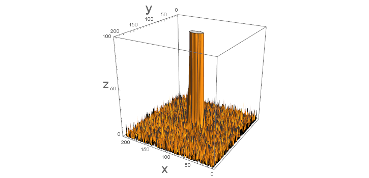
ListPlot3D[z2, PlotRange -> {All, All, {0, 100}}, BoxRatios -> {1, 1, 1}, AxesLabel -> Map[Style[#, Bold, Large] &, {"x", "y", "z"}]]
to obtain

I've truncated the z-axes to 100 to show the "noise" surrounding the "signal" in the middle. As such this is not about estimating a bivariate probability function but rather a function that has a surface similar to a bivariate normal. Because of the noise surrounding the signal I've added a constant to the original function and slightly modified the functional form for use with NonlinearModelFit.
nlm3D = NonlinearModelFit[z2, a + b Exp[-(x - mux)^2/(2 vx) - (y - muy)^2/(2 vy)],
   {{a, 25}, {b, Max[data]}, {mux, 100}, vx, {muy, 100}, vy}, {x, y}]
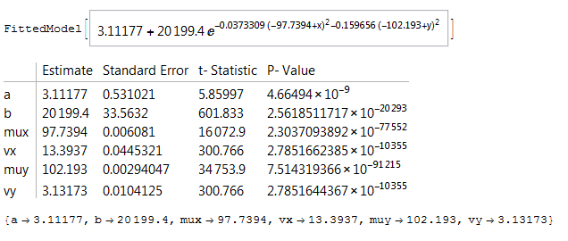
nlm3D["ParameterTable"]
estimates = nlm3D["BestFitParameters"]
with output

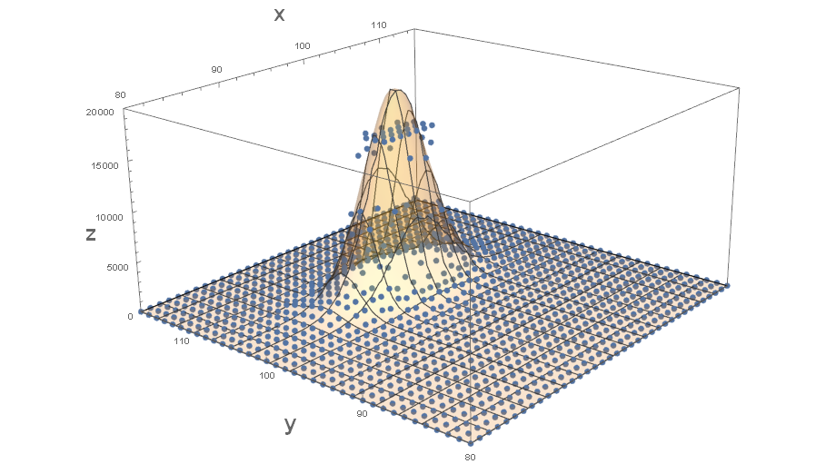
The following creates a visual assessment of the fit around the signal:
p1 = ListPointPlot3D[z2,
   PlotRange -> {{80, 115}, {80, 115}, {0, 20000}},
   BoxRatios -> {1, 1, 0.5},
   AxesLabel -> Map[Style[#, Bold, Large] &, {"x", "y", "z"}],
   PlotStyle -> PointSize[0.01]];
p2 = Plot3D[
   a + b Exp[-(x - mux)^2/(2 vx) - (y - muy)^2/(2 vy)] /. estimates, {x, 80, 115}, {y, 80, 115},
   PlotRange -> {{80, 115}, {80, 115}, {0, 20000}},
   PlotStyle -> Opacity[0.2]];
Show[{p1, p2}]

It sure seems like there is truncation for the higher values. Whether or not this is an adequate fit depends on your objective.