I can see calculating both as a quality assurance check. But if they differ by any amount (even a small amount), then why would you choose one over the other? My point is that your objective (prior to looking at the fit) should be used to decide which number to use. Otherwise you just have two different estimates.

NIntegrate would likely be more successful. But with such a dense a 202x202 array (and that the fit doesn't match the truncation at the highest values), why not just sum over the values? Your objective needs to be known to help further.

Using the 202x202 dataset I use the following:

data = Import["Z2c.dat"];
z2 = Flatten[Table[{x, y, data[[x, y]]}, {x, 202}, {y, 202}], 1];
ListPlot3D[z2, PlotRange -> {All, All, {0, 100}}, BoxRatios -> {1, 1, 1}, AxesLabel -> Map[Style[#, Bold, Large] &, {"x", "y", "z"}]]

to obtain

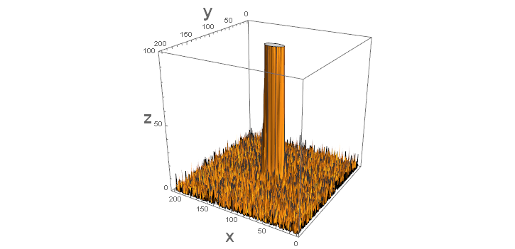
I've truncated the z-axes to 100 to show the "noise" surrounding the "signal" in the middle. As such this is not about estimating a bivariate probability function but rather a function that has a surface similar to a bivariate normal. Because of the noise surrounding the signal I've added a constant to the original function and slightly modified the functional form for use with NonlinearModelFit.

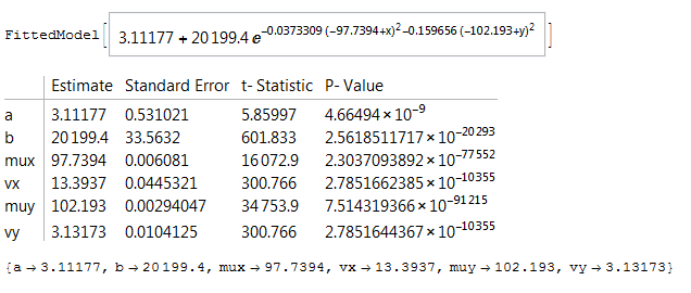
nlm3D = NonlinearModelFit[z2, a + b Exp[-(x - mux)^2/(2 vx) - (y - muy)^2/(2 vy)],
   {{a, 25}, {b, Max[data]}, {mux, 100}, vx, {muy, 100}, vy}, {x, y}]
nlm3D["ParameterTable"]
estimates = nlm3D["BestFitParameters"]

with output

The following creates a visual assessment of the fit around the signal:

p1 = ListPointPlot3D[z2, 
   PlotRange -> {{80, 115}, {80, 115}, {0, 20000}}, 
   BoxRatios -> {1, 1, 0.5}, 
   AxesLabel -> Map[Style[#, Bold, Large] &, {"x", "y", "z"}], 
   PlotStyle -> PointSize[0.01]];
p2 = Plot3D[
   a + b Exp[-(x - mux)^2/(2 vx) - (y - muy)^2/(2 vy)] /. estimates, {x, 80, 115}, {y, 80, 115}, 
   PlotRange -> {{80, 115}, {80, 115}, {0, 20000}}, 
   PlotStyle -> Opacity[0.2]];
Show[{p1, p2}]

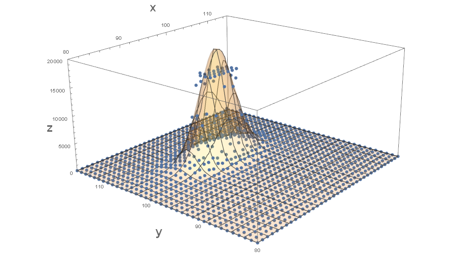
It sure seems like there is truncation for the higher values. Whether or not this is an adequate fit depends on your objective.

I suspect that the initial issue with NonlinearModelFit is that your data is not in the correct format. The following might be considered:

data = Import["Z2.dat"];
z2 = Flatten[Table[{x, y, data[[x, y]]}, {x, 202}, {y, 101}], 1];

This gets you a 20,402 x 3 array (which is what NonlinearModelFit expects: {x,y,z} are the 20,402 "data points") rather than a 202 x 101 array. I would also suggest keeping your variables in lowercase (as all of Mathematical functions start in uppercase) and avoiding subscripts (unless there is some very special need for formatting purposes).

I've just used the indices for the values of x and y as I can't tell what those should be from your dataset.

How would it be if I want to use FindFit for this matter?

Hi,

you might want to try EstimatedDistribution instead. I don't have your data, but in the documentation they do fit a multivariate distribution.

bndata = RandomVariate[BinormalDistribution[{1, 2}, {1/3, 4}, 3/4], 1000];
dist = EstimatedDistribution[bndata, BinormalDistribution[{Subscript[\[Mu], 1], Subscript[\[Mu], 2]}, {Subscript[\[Sigma], 1], Subscript[\[Sigma], 2]}, \[Rho]]]

Cheers,

Marco