In this post I will use data from NASA's ECCO2 project (http://ecco2.jpl.nasa.gov/) to simulate various scenarios: the movement of radioactive particles from the Fukushima nuclear power plant and the accumulation of rubbish in the oceans. I download about 20 years worth of oceanographic data and study how the flow of water might transport particles. A slight modification of the program might be useful to determine the crash site of Malaysian airplane MH370. The work was done with Bjoern Schelter, who is member of this community.
We will first download the vector fields for u and v direction. We obtain data for different depth, but I will only use surface currents. We first generate a list of filenames.
filenamesU = ("http://ecco2.jpl.nasa.gov/opendap/data1/cube/cube92/lat_lon/quart_90S_90N/UVEL.nc/UVEL.1440x720x50." <> # <> ".nc.ascii?UVEL[0:1:0][0:1:0][0:1:719][0:1:1439]" & /@ (StringJoin[{ToString[#[[1]]], StringTake[StringJoin[ToString /@ PadLeft[{#[[2]]}, 2]], -2], StringTake[StringJoin[ToString /@ PadLeft[{#[[3]]}, 2]], -2]}] & /@ Table[Normal[DatePlus[DateObject[{1992, 1, 2}], 3*n]], {n, 0, 2556}]));

filenamesV = ("http://ecco2.jpl.nasa.gov/opendap/data1/cube/cube92/lat_lon/quart_90S_90N/VVEL.nc/VVEL.1440x720x50." <> # <> ".nc.ascii?VVEL[0:1:0][0:1:0][0:1:719][0:1:1439]" & /@ (StringJoin[{ToString[#[[1]]], StringTake[StringJoin[ToString /@ PadLeft[{#[[2]]}, 2]], -2],StringTake[StringJoin[ToString /@ PadLeft[{#[[3]]}, 2]], -2]}] & /@ Table[Normal[DatePlus[DateObject[{1992, 1, 2}], 3*n]], {n, 0, 2556}]));
These filenames cover a time interval from the beginning of 1992 to 2012. We then download the actual data (which can take really long):
Monitor[For[k = 1, k <= Length[filenamesV], k++,
  Export["~/Desktop/OceanVelocities/velV" <> ToString[k] <> ".csv",
   ToExpression[StringSplit[StringSplit[#, "],"][[2]], ","]] & /@
    StringSplit[Import[filenamesV[[k]]], "VVEL.VVEL[VVEL.TIME="][[
     2 ;;]] ]],
 ProgressIndicator[Dynamic[k], {0, Length[filenamesV]}]]
and
Monitor[For[k = 1, k <= Length[filenamesU], k++,
  Export["~/Desktop/OceanVelocities/velU" <> ToString[k] <> ".csv",
   ToExpression[StringSplit[StringSplit[#, "],"][[2]], ","]] & /@
    StringSplit[Import[filenamesU[[k]]], "UVEL.UVEL[UVEL.TIME="][[
     2 ;;]] ]],
 ProgressIndicator[Dynamic[k], {0, Length[filenamesU]}]]
This will download about 16GB worth of data. You will, however, get reasonable results if you only use 30 frames, i.e. if you substitute Length[filenamesU] and Length[filenamesV] by 30. We will now create a figure for the first frame.
velV1 = Import["~/Desktop/OceanVelocities/velV1.csv"];
velU1 = Import["~/Desktop/OceanVelocities/velU1.csv"];
We can now generate the velocity vectors for each point on the surface of the earth
veltot = Table[{velU1[[i, j]], velV1[[i, j]]}, {i, 1, 720}, {j, 1, 1440}];
and then clean the data
veltot2 = Table[If[((StringQ[#[[1]]] || StringQ[#[[2]]]) & /@ {veltot[[i, j]] })[[1]], {0., 0.}, {velU1[[i, j]], velV1[[i, j]]}], {i, 1, 720}, {j, 1, 1440}];
We can also calculate the speed at each point.
veltottot = Table[If[((StringQ[#[[1]]] || StringQ[#[[2]]]) & /@ {veltot[[i, j]] })[[1]], 0., Norm[{velU1[[i, j]], velV1[[i, j]]}]], {i, 1, 720}, {j, 1, 1440}];
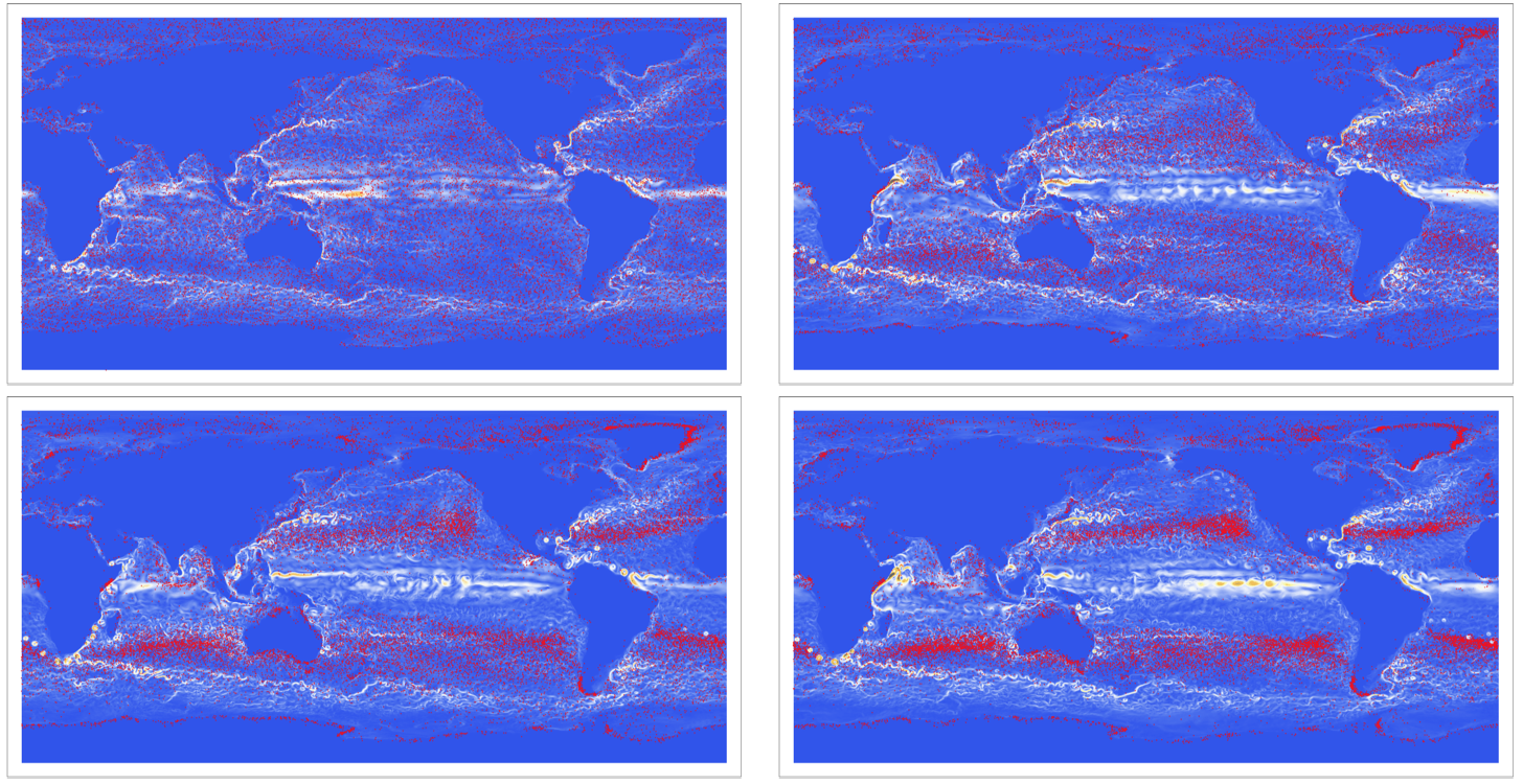
This next function will produce a visualisation of the speed profile for the first frame.
Show[ArrayPlot[Reverse[veltottot], PlotLegends -> Automatic, ImageSize -> Full, ColorFunction -> "TemperatureMap"], ListVectorPlot[Transpose[veltot2], VectorPoints -> 50]]
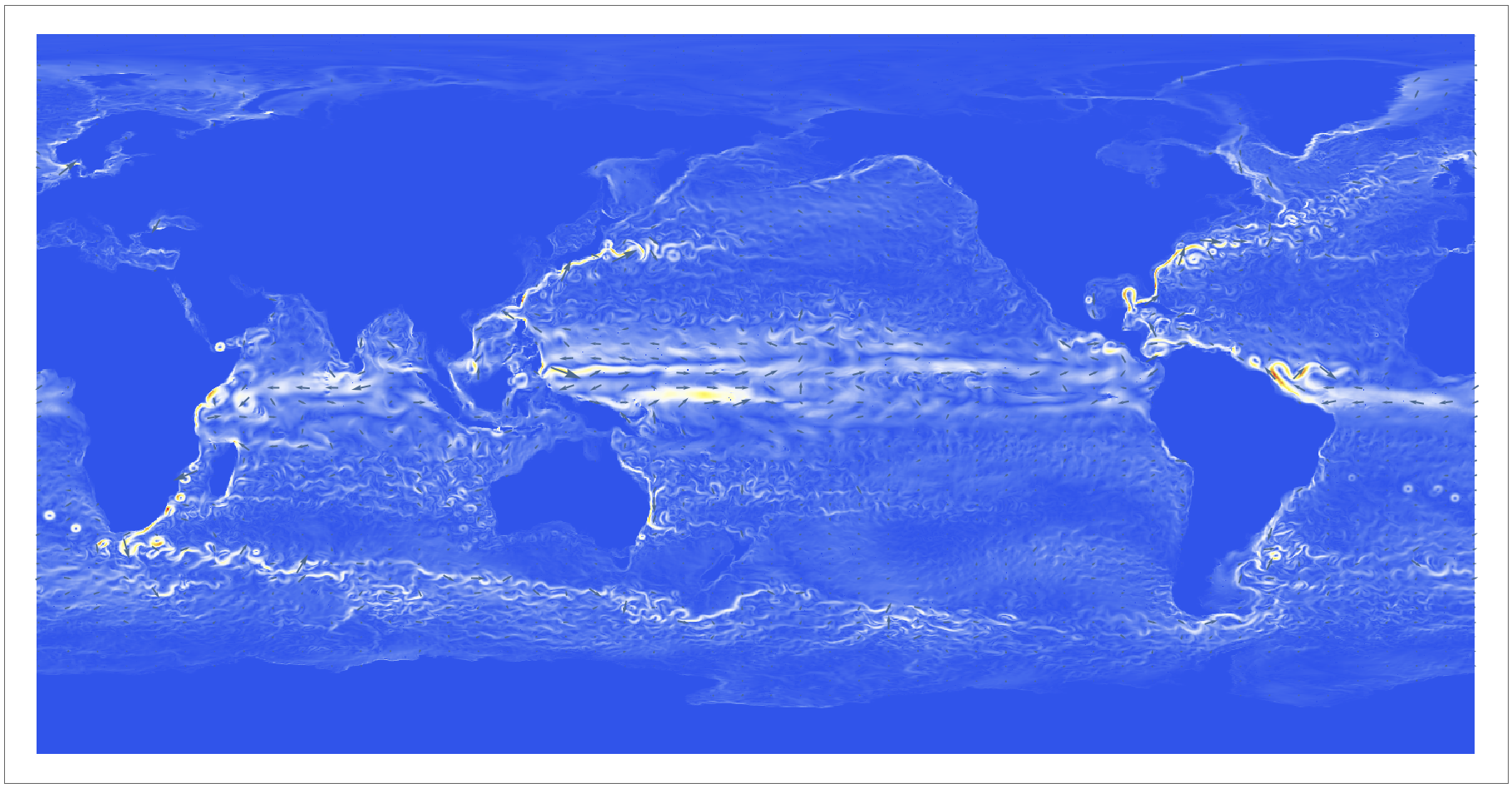
Note the incredible fine-structure in that image. We could now produce an animation for all frames. This will, however, be too large for the memory of most computers, so I would not execute it. If you only use the first 30 frames you get a reasonable idea of its working.
framesflow = {}; Monitor[
 For[k = 1, k <= Length[filenamesU], k++,
  velU1 = Import["~/Desktop/velU" <> ToString[k] <> ".csv"];
  velV1 = Import["~/Desktop/velV" <> ToString[k] <> ".csv"];
  veltot = Table[{velU1[[i, j]], velV1[[i, j]]}, {i, 1, 720}, {j, 1, 1440}];
  AppendTo[framesflow, ArrayPlot[Reverse[Table[If[((StringQ[#[[1]]] || StringQ[#[[2]]]) & /@ {veltot[[i,j]] })[[1]], 0., Norm[{velU1[[i, j]], velV1[[i, j]]}]], {i, 1, 720}, {j, 1, 1440}]], PlotLegends -> Automatic, ImageSize -> Full, ColorFunction -> "TemperatureMap"]]], k];
This following command exports all the frames as individual gif files, which can later be combined into a gif animation.
Monitor[For[k = 1, k <= Length[filenamesU], k++,
   velU1 = Import[
     "~/Desktop/OceanVelocities/velU" <> ToString[k] <> ".csv"];
   velV1 = Import[
     "~/Desktop/OceanVelocities/velV" <> ToString[k] <> ".csv"];
   veltot =
    Table[{velU1[[i, j]], velV1[[i, j]]}, {i, 1, 720}, {j, 1, 1440}];
   Export["~/Desktop/MovieOut/frame" <> ToString[1000 + k] <> ".gif",
    ArrayPlot[Reverse[Table[If[((StringQ[#[[1]]] || StringQ[#[[2]]]) & /@ {veltot[[i,j]] })[[1]], 0., Norm[{velU1[[i, j]], velV1[[i, j]]}]], {i, 1, 720}, {j, 1, 1440}]], PlotLegends -> None, ImageSize -> {1440, 730}, ColorFunction -> "TemperatureMap"]]], k];
Another advantage of saving the frames is that we can use them as background for various scenarios and thereby decrease our computation time substantially. Here is a short animation of the first couple of frames.
Now we get the trajectories of radioactive particles that are released into the ocean at the approximate site of the Fukushima power plant. We make the assumption that the particles simply follow the flow. Also, we use the vectorfield starting on 2nd January 1992. The overall patterns of the ocean currents seem to be reasonably stable over the years so that for this conceptual study this assumption will have to suffice. It is of course easy to adapt to the actual date.
We first need to introduce a formula to convert the data grid to the surface of the earth.
ClearAll["Global`*"];
f[teta_, r_, vx_, vy_] := {vx/(r*Sin[2*Pi*teta/4./360.]*2*Pi/360/4)*24*3600, vy/(N[r*2*Pi/360/4])*24*3600};
teta = 1; r = 6360000;
We now place 20000 particle into the see close to the location of Fukushima. We add a small random number to the position to model a "cloud" of particles.
teilreinpos =
 Table[{3, 511 + RandomVariate[NormalDistribution[0., 1.]], 568 + RandomVariate[NormalDistribution[0., 1.]]}, {m, 1, 20000}];
This is the main part of the program. We use the velocity to update the position of the particles. We then use the back-ground frames generated above and overlay the particle positions.
trajectories = {teilreinpos};
Monitor[Do[
   velVt = Table[
     If[StringQ[#],
          0.1*(ToExpression[#[[
                 3]]]*10^(ToExpression[#[[1]]]) ) & /@ {
            StringSplit[#, {" ", "*"}]}, 1.*#] & /@ # & /@
      Import["~/Desktop/OceanVelocities/velV" <> ToString[k] <>
        ".csv", "CSV"], {k, i - 2, i + 2}];
   velUt =
    Table[If[StringQ[#],
          0.1*(ToExpression[#[[
                 3]]]*10^(ToExpression[#[[1]]]) ) & /@ {
            StringSplit[#, {" ", "*"}]}, 1.*#] & /@ # & /@
      Import["~/Desktop/OceanVelocities/velU" <> ToString[k] <>
        ".csv", "CSV"], {k, i - 2, i + 2}];
   xfunc = ListInterpolation[velUt, {{1, 5}, {0, 720}, {0, 1440}}];
   yfunc = ListInterpolation[velVt, {{1, 5}, {0, 720}, {0, 1440}}];
   AppendTo[trajectories,
    Nest[({#[[1]], Mod[#[[2]], 720],
           Mod[#[[3]], 1440]}) & /@ (# + {0.1,
            0.1*f[#[[2]], r, xfunc[#[[1]] - i + 3., #[[2]], #[[3]]],
               yfunc[#[[1]] - i + 3., #[[2]], #[[3]]]][[2]] ,
            0.1*f[#[[2]], r, xfunc[#[[1]] - i + 3., #[[2]], #[[3]]],
               yfunc[#[[1]] - i + 3., #[[2]], #[[3]]]][[1]] } &) , # ,
        10] & /@ trajectories[[-1]]];
   Export["~/Desktop/OilSpillFrames/frame" <> ToString[1000 + i] <>
     ".gif", Show[
     Import["~/Desktop/MovieOut/frame" <> ToString[1000 + i] <>
       ".gif"],
     Graphics[{Red, Disk[#, 1]} & /@ (0.9361111 # + {44., 28.} & /@
         trajectories[[i - 2, All, {3, 2}]]),
      PlotRange -> {{0, 1440}, {0, 720}}]]];
   , {i, 3, 1238}], i];
Here are a couple of frames:
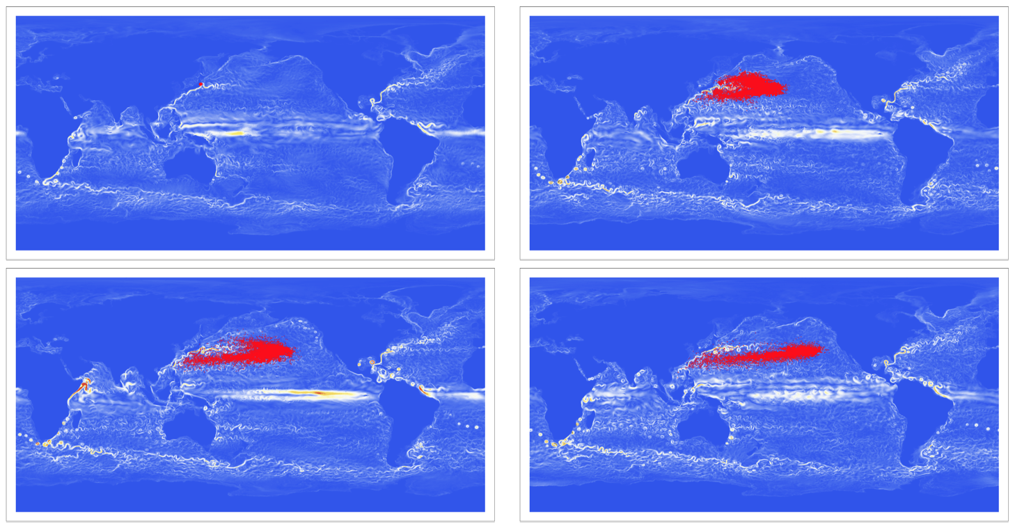
All frames yield the following animation.
Also see the higher quality animation on Youtube. https://youtu.be/8icgMg6lt0Y
Similarly we can study where rubbish, such as plastic bags would accumulate in the oceans due to the currents; these are also called gyres of marine debris particles. See also this link.
We start out just like for the Fukushima simulation:
ClearAll["Global`*"];
f[teta_, r_, vx_, vy_] := {vx/(r*Sin[2*Pi*teta/4./360.]*2*Pi/360/4)*24*3600, vy/(N[r*2*Pi/360/4])*24*3600};
teta = 1; r = 6360000;
In this case we have to distribute the particles randomly in all oceans. So I will basically distribute them everywhere and then ingore the ones over land mass, by checking whether the background flow speed is zero. So we first calculate the speed.
velVt = Table[
   If[StringQ[#],
        0.1*(ToExpression[#[[3]]]*10^(ToExpression[#[[1]]]) ) & /@ {
          StringSplit[#, {" ", "*"}]}, 1.*#] & /@ # & /@
    Import["~/Desktop/OceanVelocities/velV" <> ToString[k] <> ".csv",
     "CSV"], {k, 3 - 2, 3 + 2}];
velUt = Table[
   If[StringQ[#],
        0.1*(ToExpression[#[[3]]]*10^(ToExpression[#[[1]]]) ) & /@ {
          StringSplit[#, {" ", "*"}]}, 1.*#] & /@ # & /@
    Import["~/Desktop/OceanVelocities/velU" <> ToString[k] <> ".csv",
     "CSV"], {k, 3 - 2, 3 + 2}];

xfunc = ListInterpolation[velUt, {{1, 5}, {0, 720}, {0, 1440}}];
yfunc = ListInterpolation[velVt, {{1, 5}, {0, 720}, {0, 1440}}];
We then distribute the particles everywhere
teilreinpospre = Table[{3, RandomReal[{0, 720}], RandomReal[{0, 1440}]}, {k, 1, 30000}];
and delete the particles with zero-speed-background.
teilreinpos = Select[teilreinpospre, xfunc[3, #[[2]], #[[3]]] != 0. && yfunc[3, #[[2]], #[[3]]] != 0. &];
Now we iterate as before.
trajectories = {teilreinpos};
Monitor[Do[
   velVt = Table[
     If[StringQ[#],
          0.1*(ToExpression[#[[
                 3]]]*10^(ToExpression[#[[1]]]) ) & /@ {
            StringSplit[#, {" ", "*"}]}, 1.*#] & /@ # & /@
      Import["~/Desktop/OceanVelocities/velV" <> ToString[k] <>
        ".csv", "CSV"], {k, i - 2, i + 2}];
   velUt =
    Table[If[StringQ[#],
          0.1*(ToExpression[#[[
                 3]]]*10^(ToExpression[#[[1]]]) ) & /@ {
            StringSplit[#, {" ", "*"}]}, 1.*#] & /@ # & /@
      Import["~/Desktop/OceanVelocities/velU" <> ToString[k] <>
        ".csv", "CSV"], {k, i - 2, i + 2}];
   xfunc = ListInterpolation[velUt, {{1, 5}, {0, 720}, {0, 1440}}];
   yfunc = ListInterpolation[velVt, {{1, 5}, {0, 720}, {0, 1440}}];
   AppendTo[trajectories,
    Nest[({#[[1]], Mod[#[[2]], 720],
           Mod[#[[3]], 1440]}) & /@ (# + {0.1,
            RandomVariate[NormalDistribution[0., 0.05]] +
             0.1*f[#[[2]], r, xfunc[#[[1]] - i + 3., #[[2]], #[[3]]],
                yfunc[#[[1]] - i + 3., #[[2]], #[[3]]]][[2]] ,
            RandomVariate[NormalDistribution[0., 0.05]] +

             0.1*f[#[[2]], r, xfunc[#[[1]] - i + 3., #[[2]], #[[3]]],
                yfunc[#[[1]] - i + 3., #[[2]], #[[3]]]][[
               1]] } &) , # , 10] & /@ trajectories[[-1]]];
   Export["~/Desktop/Rubbish/frame" <> ToString[1000 + i] <> ".gif",
    Show[Import[
      "~/Desktop/MovieOut/frame" <> ToString[1000 + i] <> ".gif"],
     Graphics[{Red, Disk[#, 1]} & /@ (0.9361111 # + {44., 28.} & /@
         trajectories[[i - 2, All, {3, 2}]]),
      PlotRange -> {{0, 1440}, {0, 720}}]]];
   , {i, 3, 1238}], i];
Here are some frames:
This leads to the following animation (due to file size I only show a later part of the simulation).
Please have a look at the higher resolution and longer animation on Youtube.
It becomes clear that there are 5 large areas of rubbish in the oceans. This and their approximate positions are in accordance with their known positions and satellite data.
This type of simulation is very much simplified. We are making many assumptions, but by using the "observed" velocity field, we get around the fluid mechanical problems usually involved in these problems. The main idea can be used for many other problems as well. For example, we could iterate backwards to see where particles came from.
So I challenge you to simulate the following. Several fragments of the crashed Malaysian airplane have been found. Can you use the flow, invert the time direction and simulate where the parts must have come from? I wonder whether you can make better assmumptions than me (the larger fragments drift differently in the currents), and whether your point of origin correponds to mine.
I would love to hear back from you, and get ideas of how to apply this. I had a previous discussion with Vitaliy Kaurov about this, and there are certainly much nicer ways of representing the results. Any ideas are welcome.
Cheers,
Marco


