The type of boundary values (Dirichlet, von Neumann, other) depends on the PDE and the task you are solving. For use in the FEM package, you can specify the areas where the conditions are imposed just like you define regions using ImplicitRegion[] function. First it is required that you define the (whole) region on which the equation is to be solved. Then you have to impose boundary values on all the bounds surrounding the region. See if the example below is of any help (the notebook is attached):
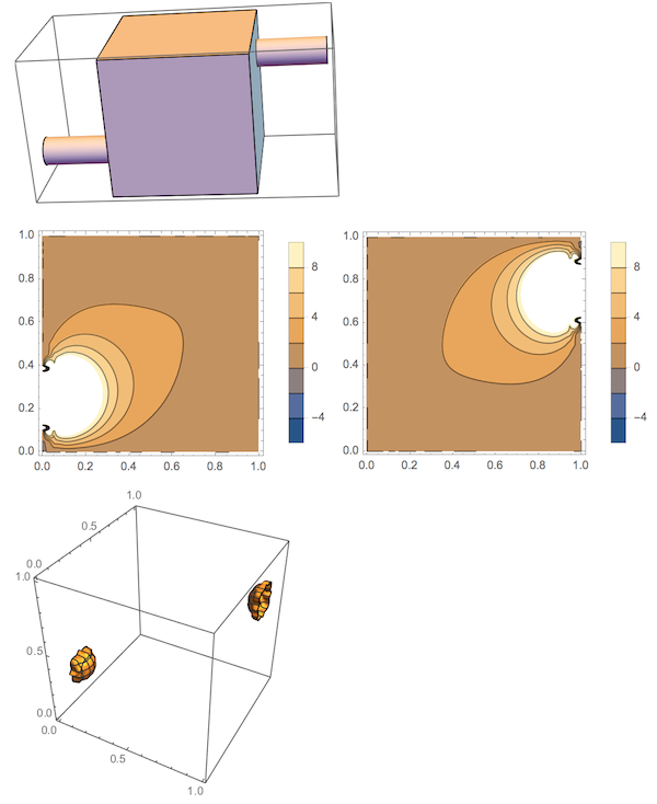
(*the situation - equation is solved only in the region of the \
cuboid, not pipes - this is just a drawing*)
ClearAll["Global`*"]
r = Cuboid[];
c1 = Cylinder[{{-0.5, 0.25, 0.25}, {0., 0.25, 0.25}}, 0.1];
c2 = Cylinder[{{1, 0.75, 0.75}, {1.5, 0.75, 0.75}}, 0.1];
Graphics3D[{r, c1, c2}]

(*solving Poisson's equation over a cube with two circled boundary \
conditions*)
\[CapitalOmega] = Cuboid[];
op = -Laplacian[u[x, y, z], {x, y, z}] - 20;
Subscript[\[CapitalGamma], D] = {
   DirichletCondition[
    u[x, y, z] ==
     200, (x == 0 && (y - 0.25)^2 + (z - 0.25)^2 <= 0.1^2) || (x ==
        1 && (y - 0.75)^2 + (z - 0.75)^2 <= 0.1^2)],(*the sources -
   areas bounded by circles*)
   DirichletCondition[
    u[x, y, z] ==
     0, (0 <= x <=
        1 && (y == 0 || z == 0 || y == 1 || z == 1)) || (x ==
        0 && (y - 0.25)^2 + (z - 0.25)^2 > 0.1^2) || (x ==
        1 && (y - 0.75)^2 + (z - 0.75)^2 >
        0.1^2)] (*rest of the walls without the areas bounded by \
circles*)
   };
uif = NDSolveValue[{op == 0, Subscript[\[CapitalGamma], D]},
   u, {x, y, z} \[Element] \[CapitalOmega]];
(*example output*)
$y1 = 0.25;
$y2 = 0.75;
ContourPlot[uif[x, $y1, z], {x, 0, 1}, {z, 0, 1},
 PlotLegends -> Automatic]
ContourPlot[uif[x, $y2, z], {x, 0, 1}, {z, 0, 1},
 PlotLegends -> Automatic]
ContourPlot3D[uif[x, y, z] == 60, {x, 0, 1}, {y, 0, 1}, {z, 0, 1}]
 Attachments:


