Message Boards Message Boards

Roads to Lyon - done in the Wolfram Language

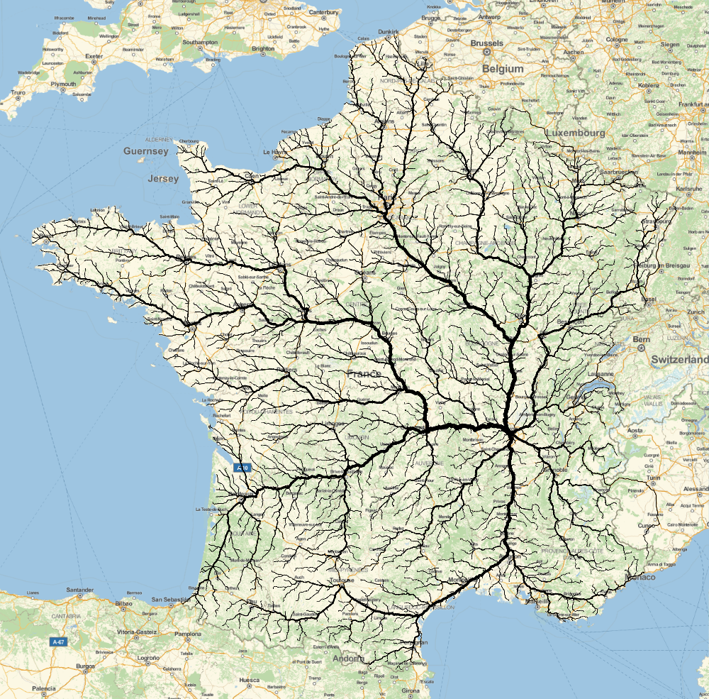
I was inspired by the Roads to Rome post (here). And wanted to check what it would look like to the town I'm living in now (Lyon, France). Here is the result and the method and code are below:
enter image description here

We first make a database of coordinates of cities in France:

SetDirectory[NotebookDirectory[]];
cities = CityData[{All, "France"}];
citiesloc = CityData[#, "Coordinates"] & /@ cities;
citiesloc = DeleteMissing[citiesloc, 1, \[Infinity]];
Export["francecities.txt", citiesloc, "Table"]

quite self-explanatory, it will save it as a table of coordinates.

Now I read those back in, and check find those that are in 'mainland' France and create a nearest-function of those coordinates:

SetDirectory[NotebookDirectory[]];
citiesloc = Import["francecities.txt", "Table"];

reg = CountryData["France", "Polygon"];
reg = Identity @@ Identity @@ reg;
reg = First@MaximalBy[reg, Length];
region = MeshRegion[reg, Polygon[Range[Length[reg]]]];
rmf = RegionMember[region];
citiesloc = Select[citiesloc, rmf];

ccf = Nearest[citiesloc];

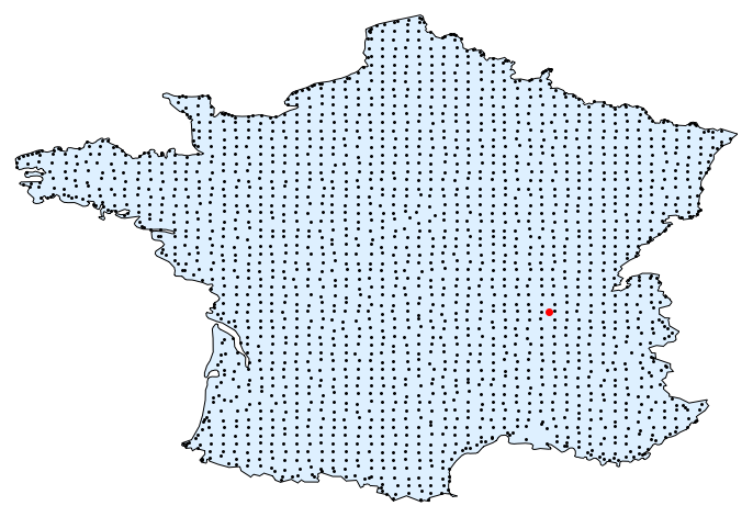
I now create a grid of points in the coordinates of france, and find for each the nearest city. I filter then any duplicates out. Lastly I show a map:

bounds = CoordinateBounds[reg];
n = {60, 60};
pts = MapThread[Subdivide[#1[[1]], #1[[2]], #2] &, {bounds, n - 1}];
pts = Tuples[pts];
pts = DeleteDuplicates[First@*ccf /@ pts];
pts // Length

(*dest=Lyon (city)["Coordinates"]*)
dest = {45.76`, 4.83`};

Graphics[{{EdgeForm[Black], FaceForm[LightBlue], Polygon[Reverse /@ reg]}, Point[Reverse /@ pts], Style[Point[Reverse@dest], Red, PointSize[Large]]}]
enter image description here

Now we have to calculate the route from any black point to Lyon (in red). This is very easy with the TravelDirections function (introduced v10.3).

ClearAll[SavePath]
SavePath[loc1:{lat_,lon_},loc2:{lat2_,lon2_},fnout_String]:=Block[{td},
 td=Check[TravelDirections[{GeoPosition[loc1],GeoPosition[loc2]}],"fail"];
 If[td=!="fail",
  td=td["TravelPath"][[1,1]];
  Export[fnout,td]
 ,
  Print["Failed "<> fnout]
 ]
]
fnsout=ToString[#]<>".wdx"&/@Range[Length[pts]];
MapThread[SavePath[#1,dest,#2]&,{pts,fnsout}]

I let it run (this goes over the internet and the Wolfram servers give us the routes back) and the routes are saved to WDX files. Sorry for overloading the servers... ~10 or so failed for whatever reason. No worries, doesn't matter so much. In total 2165 did work. Now let's plot it!

We load in all the data (and filter those out that are too small (they returned $Failed or so):

SetDirectory[NotebookDirectory[]];
$HistoryLength = 2;
fns = FileNames["*.wdx"];
alldata = Import /@ fns;
alldata = Select[alldata, ByteCount[#] > 500 &]; 

Now let's count the road pieces:

pieces = Partition[DeleteDuplicates[Flatten[#, 1]], 2, 1] & /@ alldata;
pieces = Flatten[pieces, 1];
pieces = Round[pieces 10^11];
tpieces = Tally[pieces];
tpieces = GatherBy[tpieces, Last];
tpieces = SortBy[tpieces, Part[#, 1, -1] &];
widths = tpieces[[All, 1, -1]];
tpieces = tpieces[[All, All, 1]];
tpieces = Split[#, Last[#1] == First[#2] &] & /@ tpieces;
tpieces = Map[DeleteDuplicates[Flatten[#, 1]] &, tpieces, {2}];
tpieces /= 10^11.0;

What happens here? Well, first I take every route and flatten it, remove duplicates, and then cut it up in to pieces of length 2 (Partition[...,2,1]). Then I pile up all those little pieces (line 2). Because of rounding and so on I will round the coordinates and do so by multiplying them to make it very big integers). Now I tally all the small road-pieces to see how 'busy' they are. And then I group all the road-pieces that are equally busy (GatherBy[...]). And then Sort by the busyness of it (SortBy[...]). I save the busyness for later in the variable widths. Now I drop all the busyness-values, and now make the plotting a little easier by merging pieces of road, and removing duplicates. Lastly, I undo the rounding/multiplying.

Lastly we plot the result:

GeoGraphics[MapThread[{Thickness[0.0008 #1^0.3], GeoPath[#2, "TravelPath"]} &, {widths, tpieces}], ImageSize -> 1000]

enter image description here

Looks pretty cool! I just wanted to share this because it is (to me at least) really amazing that you can just do this within 50 lines or so and it took me 30 minutes or so to write it! Imagine doing this in C, Python, Java, Swift, ....!

POSTED BY: Sander Huisman
13 Replies
Posted 6 years ago

I tried Sander's code for the initial post. (In Mathematica 12.) Everything worked fine up to the last step when it seemed to mess up plotting some of the routes. Maybe some change has broken the code. I found that it can be fixed by plotting the road segments individually. In the last line, replace

GeoPath[#2, "TravelPath"]

with

Map[GeoPath, #2]

I also found that the rounding strategy was not necessary. First, I experimented with just truncating the data to 5 decimal places, which seemed fine. Then when I produced a tidied up copy in a separate notebook, I forgot to include that step, and it was still fine. This was for the UK, with a grid of only 30x30. Whether it would be ok elsewhere, I don't know. This allowed simplification of the final steps, and I dispensed with the intermediate saving to disk. The grid for the UK came out not as regular as for France, with various empty spaces in the Scottish Highlands for example. My final code, for my town, was:

num = 30; country = "UnitedKingdom"; dest = 
 CityData[{"Bourne", "Lincolnshire", "UnitedKingdom"}, "Coordinates"];
a = 0.5; (*affects how the road width scales*)
cities = CityData[{All, country}];
citiesloc = CityData[#, "Coordinates"] & /@ cities;
citiesloc = DeleteMissing[citiesloc, 1, \[Infinity]];
reg = CountryData[country, "Polygon"];
reg = Identity @@ Identity @@ reg;
reg = First@MaximalBy[reg, Length];
region = MeshRegion[reg, Polygon[Range[Length[reg]]]];
rmf = RegionMember[region];
citiesloc = Select[citiesloc, rmf];
ccf = Nearest[citiesloc];
bounds = CoordinateBounds[reg];
n = {num, num};
pts = MapThread[Subdivide[#1[[1]], #1[[2]], #2] &, {bounds, n - 1}];
pts = Tuples[pts];
pts = DeleteDuplicates[First@*ccf /@ pts];
pts // Length;
Graphics[{{EdgeForm[Black], FaceForm[LightBlue], 
   Polygon[Reverse /@ reg]}, Point[Reverse /@ pts], 
  Style[Point[Reverse@dest], Red, PointSize[Large]]}]

Then...

routes = Map[{dest, #} &, pts];
td = Map[TravelDirections[GeoPosition /@ #] &, routes];
td = DeleteCases[td, $Failed];
tp = Map[#["TravelPath"][[1, 1]] &, td];
pieces = Map[Partition[DeleteDuplicates[Flatten[#, 1]], 2, 1] &, tp];
pieces = Flatten[pieces, 1];
tpieces = Tally[pieces];
tpieces = GatherBy[tpieces, Last];
tpieces = SortBy[tpieces, Part[#, 1, -1] &];
widths = tpieces[[All, 1, -1]];
tpieces = tpieces[[All, All, 1]];
GeoGraphics[
 MapThread[{Thickness[#1^a/1000], Map[GeoPath, #2]} &, {widths,
    tpieces}], GeoRange -> Entity["Country", country]]

And here is the result:

Roads to Bourne

POSTED BY: Marc Widdowson

enter image description here - another post of yours has been selected for the Staff Picks group, congratulations !

We are happy to see you at the tops of the "Featured Contributor" board. Thank you for your wonderful contributions, and please keep them coming!

POSTED BY: EDITORIAL BOARD

Realy cool! Beautiful post! I suggest you to use some compression in your file, they are too big. Maybe something like: Export["~/desktop/test.jpg",RandomImage[], "CompressionLevel"->0.2 ]

POSTED BY: Rodrigo Murta

They were only 10-20 Megabytes each ;-) I changes them to ~4 (rather than 18) megapixel images. I didn't notice with the fast connection!

POSTED BY: Sander Huisman

Also interesting is to look at the length of the route versus the direct distance:

copy=DeleteDuplicates[Flatten[#,1]]&/@alldata; (* merge data and delete duplicates*)
directlength=GeoDistance2@@@copy[[All,{1,-1}]]; (* calculate direct distance*)
routelength=BlockMap[GeoDistance2@@#&,#,2,1]&/@copy; (* calculate road distance *)
routelength=Total/@routelength; (* total it*)
ListPlot[{directlength,routelength}\[Transpose]/1000.0,Frame->True,AspectRatio->Automatic,Epilog->{Line[{{0,0},{1000,1000}}]},FrameLabel->(Style[#,14]&/@{"Direct distance [km]","Road distance [km]"})]
Histogram[routelength/directlength,Automatic,"PDF",Frame->True,FrameLabel->(Style[#,14]&/@{"\[CurlyPhi] = Road distance/Direct distance","PDF(\[CurlyPhi])"})]

where GeoDistance2 is a quick version of GeoDistance:

ClearAll[GeoDistance2]
GeoDistance2[{lat1_,lon1_},{lat2_,lon2_}]:=Module[{\[CurlyPhi]1,\[CurlyPhi]2,\[CapitalDelta]\[CurlyPhi],\[CapitalDelta]\[Lambda],a,c},
    {\[CurlyPhi]1,\[CurlyPhi]2}={lat1,lat2}Degree;
    \[CapitalDelta]\[CurlyPhi]=\[CurlyPhi]2-\[CurlyPhi]1;
    \[CapitalDelta]\[Lambda]=(lon2-lon1)Degree;
    a=Haversine[\[CapitalDelta]\[CurlyPhi]]+Cos[\[CurlyPhi]1]Cos[\[CurlyPhi]2]Haversine[\[CapitalDelta]\[Lambda]];
    c=2ArcTan[Sqrt[1-a],Sqrt[a]];
    6.3674446571 10^6c (* result in meters *)
]

enter image description here

enter image description here

I guess the average ratio describes how developed a country is/how mountainous it is/how many water bodies it has. A comparison for different countries would be very nice. But I don't want to kill the Wolfram servers...

POSTED BY: Sander Huisman

Creating the 'normalised' paths was quite easy:

SetDirectory[NotebookDirectory[]];
$HistoryLength=2;
fns=FileNames["*.wdx"];
alldata=Import/@fns;
alldata=Select[alldata,ByteCount[#]>500&];

copy=DeleteDuplicates[Flatten[#,1]]&/@alldata;
origdirect=copy[[All,{1,-1}]];
copy=MapThread[(#1\[Transpose]-#2)\[Transpose]&,{copy,copy[[All,-1]]}]; (* subtract final destination from all points (last point for each route is 0,0 afterwards *)
rotmax=RotationMatrix[{#,{0,-1}}]&/@copy[[All,1]]; (* create rotation matrix for each route *)
copy=MapThread[With[{rm=#1,data=#2},rm.#&/@data]&,{rotmax,copy}]; (* rotate each of them *)
scale=Norm/@copy[[All,1]]; (* find the scales and rescale *)
copy/=scale;

g=Graphics[Line[copy],ImageSize->4000]; (* black lines *)
Export["NormalisedRoutes.png",g]

angdegrees=QuantityMagnitude[(GeoDirection@@@(Reverse/@origdirect)),"AngularDegrees"]; (* get angle between start and finish*)
colors=Hue/@Subdivide[0.0,1,Length[angdegrees]-1]; (* create a rainbow *)
ord=Ordering[angdegrees];
colors=colors[[ord]]; (* order the rainbox by the angle *)
g=Graphics[MapThread[{#1,Line[#2]}&,{colors,copy}],ImageSize->4000]; (* colored by direction using hue *)
Export["NormalisedRoutesColored.png",g]

enter image description here enter image description here

Looks visually very interesting!

POSTED BY: Sander Huisman

Dear Sander,

what you (and Bernat) are doing is absolutely amazing! I will study your code in detail. Thanks a lot for sharing!

... you can just do this within 50 lines or so and it took me 30 minutes or so to write it! Imagine doing this in C, Python, Java, Swift, ....!

This is more than true!

Best wishes! -- Henrik

POSTED BY: Henrik Schachner

Thanks! If you have any questions let me know. I added some comments and explanation but if you're not fluent in the WL it might be intimidating!

POSTED BY: Sander Huisman

@Sander Huisman this is wonderful work! I liked your grid a lot too - good visual aid to understand the scales of computation. This, I bet, will get many readers and some might miss another nice visual explanation from the authors of original project. The explanation is a bit buried on their site. It also relates to what @Marco Thiel is suggesting, which is indeed an interesting direction of thinking. So here are a few images and quotes from the authors of the original project:

The idea behind the "Urban Mobility Fingerprint" is to calculate routes to a single destination (A) from many departure points (B). The points (B) are located on a radius around the destination. The size of the radius is defined by travel time with different transportation modes. All routes together then create the "Urban Mobility Fingerprint".

enter image description here

Once the routes are drawn, all starting points are rotated and align on to one ideal connection line. The direct line between these two dots is the ideal connection between the two locatoins. The length of the routes is scaled to fit the connecting ideal line. We call the graph that is created the "Street DNA". Since in reality street connections never follow a perfectly straight line deviations are unavoidable. The Street DNA graph shows exaclty these situations. The color-coding helps to identify in what compass direction routes are located on the map. The outline is created by connecting all locations (B) that are reached within the same travel time. These lines are called isochrones. The color of each route is defined by the compass direction it leads to, making it easier to relate routes within the fingerprint graph. We created the Urban Mobility Fingerprint and Street DNA graphs for a couple of cities around the world. The 13 examples we selected are supposed to resemble a lage diversity of culutral backrounds around the globe combined with objectivly compelling street networks. Next to different cultural backgrounds, we also looked for characteristic places and iconic street topography. Coastal locations like San Fransisco, Dubai's Palm Island or Manhanttan show the extreme deviations from the ideal connection we experience while travelling through our cities.

enter image description here

POSTED BY: Vitaliy Kaurov

Dear Vitaliy,

for intra-city travel the function I posted here might be useful. The problem is that it uses the GoogleMaps API and only allows us to use a limited number of requests per day.

Cheers,

Marco

POSTED BY: Marco Thiel

Creating these lines for the routes on a country-scale should be quite easy; just some rotation and scaling. I'll give it a try later. I chose a grid of cities rather than all cities so that it is more homogeneously distributed over the area, and thus not biasing certain areas.

Thanks for the nice comments!

POSTED BY: Sander Huisman

Dear Sander,

very nice indeed. As I said in Bernat's post, I am still running his simulation, but It might be really interesting to colour the individual "branches" according to their "travel time distance" (as opposed to just distance) to Lyon. So using a colour gradient to indicate travel time from that point to Lyon. I have been playing around with that in combination with other means of transport. Say you have the road network, but also a air travel network. The travel time from Heathrow to Amsterdam could be shorter than the travel time from Heathrow to some parts of London!

Unfortunately, my results are not yet good enough to be posted...

Cheers,

Marco

PS: Very good job on the GCHQ Christmas Puzzle by the way!
PPS: It appears that you have 1500+ views in about an hour. Quite impressive.

POSTED BY: Marco Thiel

Hi Marco,

Thanks for the kind words. Unfortunately I didn't save the times. But should be also possible. I might try tonight. Just to clarify: I'm also not using the distance now. I just color it by how often a piece of road is 'used' by all the routes. But it might be interesting to see it as a graph indeed. I will dig deeper later...

thanks!

POSTED BY: Sander Huisman
Reply to this discussion
Community posts can be styled and formatted using the Markdown syntax.
Reply Preview
Attachments
Remove
or Discard

Group Abstract Group Abstract