Easy Cube is a reflexion game from Japan. It consists of a set of 7 pieces which are "tetris"-like (each piece is a simple geometrical shape made from 3,4 or 5 cubes), and a collection of 48 problems, where the goal is to use the pieces to fill a given shape (in 2d, or in 3d for the hardest problems).
The game box 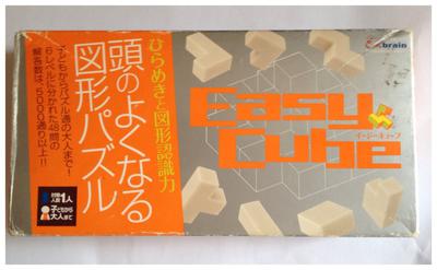
The 7 pieces 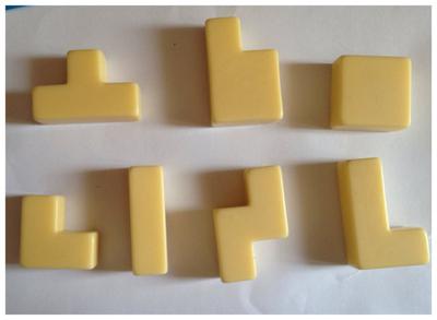
2 examples of problems 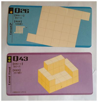
It is pleasant to play, with the difficulty slowly increasing whit the hardest problems. I decided to try to solve it using Mathematica. I did not use any advanced mathematics for this (which anyway I would not know :-)), and I wanted a method general enough so it could solve all the problems without any specific adpatation. I went for a purely random method, where the program places a first piece at random, then try to put a second piece, etc. When it fails to add a piece after a fixed number of attemps, it simply starts the whole process again. So this program does not learn anything... It just tries many many different possibilities, until it finds a solution ! Using Wolfram language, the code to make it and to vizualize to result was quite simple and effective (I show the code details at the end of this post for people interested). In particular, going from the 2d case to the 3d case needed very small changes only.
The two followings animations show the program in action for a 2d problem and a 3d problem 
The number of attempts needed to reach a solution is of course random, and depends on the difficulty of the problem. Typically, it takes between a few hundreds and a few thousands iterations, which takes between a few seconds to 1-2 minutes. Here a sample of 4 solutions found for a 2d problem : 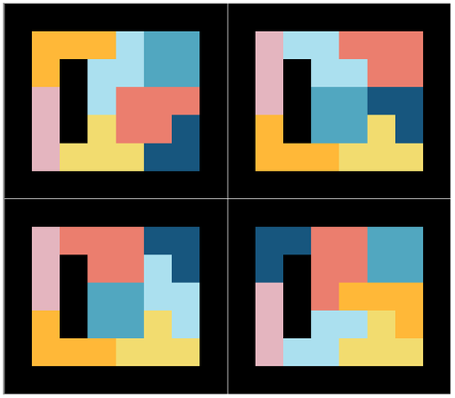
And 2 solutions from a 3d problem : 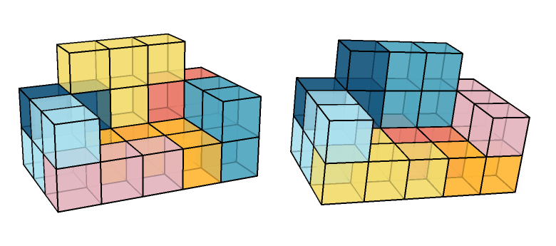
Finally, I considered it if was possible to use this method to find all solutions for a given problem (the number of different solutions is an info given on the description of each problem). In principle, because the method is random, it is not well suited for this (one can never be sure that all solutions have been found). However, since the method is quite fast, I decided to try anyway. For a given problem, I computed 10000 solutions. Here is a plot of the number of attempts needed for each solution, and a histogram of this: 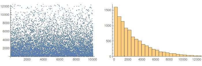
On average, finding a solution to this problem requested 2882 attempts...
From the 10000 solutions, one wants only different solutions. This is easily done with the DeleteDuplicates command:
SolgridQ26ListMReduced =
 DeleteDuplicates@SolgridQ26ListM; Length@SolgridQ26ListMReduced

362
which gives 362 different solutions. However, since this problem geometry has a simple central symmetry, one also want to get rid of "symmetric copies" of the solutions. Defining the symmetry operation as the GsymGrid function, this is again done with a DeleteDuplicates command :
SolgridQ26ListMReducedSym =
 DeleteDuplicates[
  SolgridQ26ListMReduced, #2 ==
    GSymGrid[#1] &]; Length@SolgridQ26ListMReducedSym

188
which gives 188 unique solutions. This is precisely the number which is given in the problem description ! So the method was able to find all solutions. Here is plot with the 188 solutions: 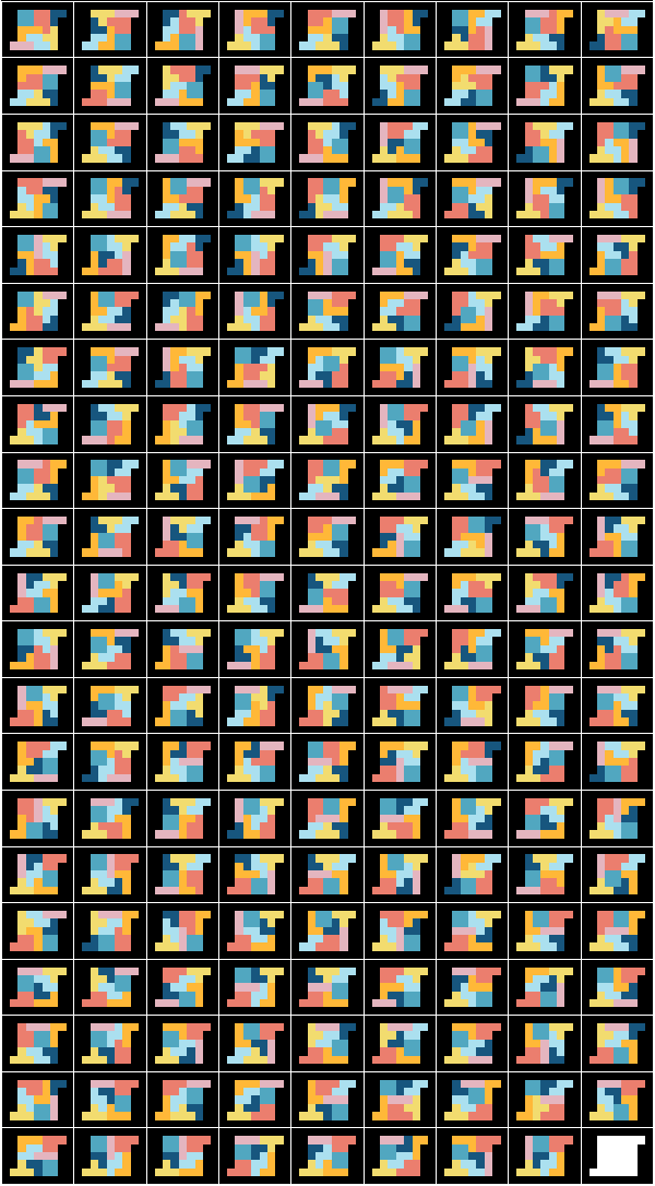
Details of the code
Definition of the pieces (2d case). Each piece is a simple list of the points make the piece. When then construct, for each piece, a list of copies of it with all possible orientations.
Pieces Definitions
PTriangle = {{0, 0}, {0, 1}, {1, 0}};
PSquare = {{0, 0}, {0, 1}, {1, 0}, {1, 1}};
PLine = {{0, 0}, {0, 1}, {0, 2}};
PL = {{0, 0}, {0, 1}, {1, 0}, {2, 0}};
PPodium = {{0, 0}, {0, 1}, {-1, 0}, {1, 0}};
PSnake = {{0, 0}, {0, 1}, {1, 0}, {-1, 1}};
PBulky = {{0, 0}, {1, 0}, {0, 1}, {1, 1}, {-1, 1}};
(* Rotation by angle \[Pi]/2 matrix*)
Mrot = {{0, 1}, {-1, 0}};
(* Reflection by y-axis matrix *)
Mref = {{-1, 0}, {0, 1}};
MUnit = {{1, 0}, {0, 1}};
(*Operators which perform a given number of rotation, and of \
reflection*)
RotatePiece[piece_, n_] := Nest[Mrot.# &, #, n] & /@ piece
ReflectPiece[piece_, n_] :=
 If[n == 0, (MUnit.#) & /@ piece, (Mref.#) & /@ piece]
Each piece with all the possible orientations
PTriangleAll = {PTriangle, RotatePiece[PTriangle, 1],
   RotatePiece[PTriangle, 2], RotatePiece[PTriangle, 3]};
PSquareAll = {PSquare};
PLineAll = {PLine, RotatePiece[PLine, 1]};
PLAll = Module[{PLr = ReflectPiece[PL, 1]}, {PL, RotatePiece[PL, 1],
    RotatePiece[PL, 2], RotatePiece[PL, 3], PLr, RotatePiece[PLr, 1],
    RotatePiece[PLr, 2], RotatePiece[PLr, 3]}];
PPodiumAll = {PPodium, RotatePiece[PPodium, 1],
   RotatePiece[PPodium, 2], RotatePiece[PPodium, 3]};
PSnakeAll = {PSnake, RotatePiece[PSnake, 1], ReflectPiece[PSnake, 1],
   RotatePiece[ReflectPiece[PSnake, 1], 1]};
PBulkyAll =
  Module[{PBulkyr = ReflectPiece[PBulky, 1]}, {PBulky,
    RotatePiece[PBulky, 1], RotatePiece[PBulky, 2],
    RotatePiece[PBulky, 3], PBulkyr, RotatePiece[PBulkyr, 1],
    RotatePiece[PBulkyr, 2], RotatePiece[PBulkyr, 3]}];
tPieces = {PBulkyAll, PLAll, PPodiumAll, PSnakeAll, PSquareAll,
   PLineAll, PTriangleAll};
tPiecesNames = {"Bu", "Ll", "Po", "Sn", "Sq", "Li", "Tr"};
Functions which place the pieces
Piece placement functions
PutPiece[piece_, piecename_, grid_] :=
 Module[{IniPt, IniPtxy, Pts, Vcheck, PtsinGrid, Pos, i, gridx},
  gridx = grid;
  IniPt = RandomChoice[Position[gridx, 0]];
  Pts = Map[IniPt + # &, RandomChoice[piece]];
  PtsinGrid = gridx[[Sequence @@ #]] & /@ Pts;
  Vcheck =
   If[PtsinGrid ==  Table[0, Length[PtsinGrid]], "success", "failure"];
  If[Vcheck == "success",
   Do[gridx[[Sequence @@ Pts[[i]]]] = piecename, {i,
     Length[Pts]}]; {"success", gridx}, {"failure", gridx}]
  ]
AddOnePiece[gridin_, piece_, piecename_, nmax_] :=
 Module[{cc = "failure", nn = 0, aa},
  While[(cc != "success") && (nn < nmax),
   aa = PutPiece[piece, piecename, gridin]; cc = aa[[1]];
   nn = nn + 1]; aa]
Grid definition, and plotting functions The initial grid is a ensemble of 0, embedded in a series of 1, forming a matrix. When a piece is placed the 0's it occupies are replaced by the name of the piece
General Grid Definitions
TheGrid0 = Table[1, {i, -6, 6, 1}, {j, -6, 6, 1}];
GridDefine[coord_] :=
 Module[{gridout}, gridout = TheGrid0;
  Do[gridout[[Sequence @@ (coord[[i]] + {7, 7}) ]] = 0, {i,
    Length[coord]}]; gridout]
DrawPieceRectangle[piecename_, grid_, color_] := {color,
  Map[Rectangle[{#[[1]] - 0.5 - 7, #[[2]] - 0.5 - 7}, {#[[1]] + 0.5 -
       7, #[[2]] + 0.5 - 7}, RoundingRadius -> 0.] &,
   Position[grid, piecename]]}
mycolors = ColorData[24];
PlotGrid[grid_, plotrange_] :=
 Graphics[{{White, Rectangle[{-6, -6}, {6, 6}]},
   DrawPieceRectangle[0, grid, White],
   DrawPieceRectangle[1, grid, Black],
   DrawPieceRectangle[tPiecesNames[[#]], grid,
      mycolors[If[# != 6, #, # + 4]]] & /@ Range[7]},
  PlotRange -> plotrange]
The final solving functions
Full solving function
Get the solution, and at each step provides a plot named p, which can be dynamically visualized using a cell with Dynamic[p]
SolveGrid[InitGrid_, plotrange_] :=
 Module[{imax, nattempt, grid, i, vc}, imax = 0; nattempt = 0;
  While[imax < 8, grid[1] = InitGrid; i = 1; vc = "success";
   While[(i < 8) && (vc == \!\(\*
TagBox[
StyleBox["\"\<success\>\"",
ShowSpecialCharacters->False,
ShowStringCharacters->True,
NumberMarks->True],
FullForm]\)),
     {vc, grid[i + 1]} =
     AddOnePiece[grid[i], tPieces[[i]], tPiecesNames[[i]], 30];
    p = PlotGrid[grid[i + 1], plotrange];
    If[vc == "success" || i < 7, i++; imax = i, i++]]; nattempt++];
  Print[nattempt]; PlotGrid[grid[8], plotrange]; grid[8]]
Get ony the solution, without final plot, nor dynamical vizualisation
SolveGridBare[InitGrid_] :=
 Module[{imax, nattempt, grid, i, vc}, imax = 0; nattempt = 0;
  While[imax < 8, grid[1] = InitGrid; i = 1; vc = "success";
   While[(i < 8) && (vc == \!\(\*
TagBox[
StyleBox["\"\<success\>\"",
ShowSpecialCharacters->False,
ShowStringCharacters->True,
NumberMarks->True],
FullForm]\)),
     {vc, grid[i + 1]} =
     AddOnePiece[grid[i], tPieces[[i]], tPiecesNames[[i]], 30];
    If[vc == "success" || i < 7, i++; imax = i, i++]]; nattempt++];
  Print[nattempt]; grid[8]]
SolveGridBare2[InitGrid_] :=
 Module[{imax, nattempt, grid, i, vc}, imax = 0; nattempt = 0;
  While[imax < 8, grid[1] = InitGrid; i = 1; vc = "success";
   While[(i < 8) && (vc == \!\(\*
TagBox[
StyleBox["\"\<success\>\"",
ShowSpecialCharacters->False,
ShowStringCharacters->True,
NumberMarks->True],
FullForm]\)),
     {vc, grid[i + 1]} =
     AddOnePiece[grid[i], tPieces[[i]], tPiecesNames[[i]], 30];
    If[vc == "success" || i < 7, i++; imax = i, i++]];
   nattempt++]; {grid[8], nattempt}]
Example of use
coordQ35 =
  Join[Table[{i, 2}, {i, -2, 3}], Table[{i, -2}, {i, -2, 3}],
   Table[{i, 1}, {i, 0, 3}], Table[{i, 0}, {i, 0, 3}],
   Table[{i, -1}, {i, 0, 3}], Table[{-2, j}, {j, -1, 1}]];

TheGridQ35 = GridDefine[coordQ35];
SolgridQ35ex1 = SolveGridBare[TheGridQ35];
PlotGrid[SolgridQ35ex1, {{-3.5, 4.5}, {-3.5, 3.5}}]
A dynamic view of the process (similar to the animations shown above) is obtained by running a cell "Dynamic[p]" before calling SolveGrid[TheGridQ35,{{-3.5, 4.5}, {-3.5, 3.5}}]
Pieces definition for the 3 case (here all the possible orientations are obtained by applying randomly rotations and reflection on the initial piece)
Pieces Definitions
PTriangle = {{0, 0, 0}, {0, 1, 0}, {1, 0, 0}};
PSquare = {{0, 0, 0}, {0, 1, 0}, {1, 0, 0}, {1, 1, 0}};
PLine = {{0, -1, 0}, {0, 0, 0}, {0, 1, 0}};
PL = {{0, 0, 0}, {0, 1, 0}, {1, 0, 0}, {2, 0, 0}};
PPodium = {{0, 0, 0}, {0, 1, 0}, {-1, 0, 0}, {1, 0, 0}};
PSnake = {{0, 0, 0}, {0, 1, 0}, {1, 0, 0}, {-1, 1, 0}};
PBulky = {{0, 0, 0}, {1, 0, 0}, {0, 1, 0}, {1, 1, 0}, {-1, 1, 0}};
(* Rotation by angle \[Pi]/2 matrix*)
Mrotz = {{0, 1, 0}, {-1, 0, 0}, {0, 0, 1}};
Mrotx = {{1, 0, 0}, {0, 0, 1}, {0, -1, 0}};
Mrotx = {{0, 0, -1}, {0, 1, 0}, {1, 0, 0}};
(* Reflection  matrix *)
Mrefx = {{-1, 0, 0}, {0, 1, 0}, {0, 0, 1}};
Mrefy = {{1, 0, 0}, {0, -1, 0}, {0, 0, 1}};
Mrefz = {{1, 0, 0}, {0, 1, 0}, {0, 0, -1}};
MUnit = {{1, 0, 0}, {0, 1, 0}, {0, 0, 1}};
(*Operators which perform a given number of rotation, and of \
reflection*)
RotatePiecex[piece_, n_] := Nest[Mrotx.# &, #, n] & /@ piece
RotatePiecey[piece_, n_] := Nest[Mrotx.# &, #, n] & /@ piece
RotatePiecez[piece_, n_] := Nest[Mrotz.# &, #, n] & /@ piece
ReflectPiecex[piece_, n_] :=
 If[n == 0, (MUnit.#) & /@ piece, (Mrefx.#) & /@ piece]
ReflectPiecey[piece_, n_] :=
 If[n == 0, (MUnit.#) & /@ piece, (Mrefy.#) & /@ piece]
ReflectPiecez[piece_, n_] :=
 If[n == 0, (MUnit.#) & /@ piece, (Mrefz.#) & /@ piece]
Each piece with all the possible orientations
MakeAllPieces[piece_] :=
 DeleteDuplicates@
  Table[Module[{Rota, Rotb, Rotc, Refa, Refb, Refc, na, nb, nc, ma,
     mb, mc},
    Rota = RandomChoice[{RotatePiecex, RotatePiecey, RotatePiecez}];
    Rotb = RandomChoice[{RotatePiecex, RotatePiecey, RotatePiecez}];
    Rotc = RandomChoice[{RotatePiecex, RotatePiecey, RotatePiecez}];
    Refa = RandomChoice[{ReflectPiecex, ReflectPiecey, ReflectPiecez}];
    Refb = RandomChoice[{ReflectPiecex, ReflectPiecey, ReflectPiecez}];
    Refc = RandomChoice[{ReflectPiecex, ReflectPiecey, ReflectPiecez}];
    na = RandomInteger[{0, 3}]; nb = RandomInteger[{0, 3}];
    nc = RandomInteger[{0, 3}];
    ma = RandomInteger[{0, 1}]; mb = RandomInteger[{0, 1}];
    mc = RandomInteger[{0, 1}];
    Refc[Rotc[Refb[Rotb[ Refa[Rota[piece, na], ma], nb], mb], nc],
     mc]], {i, 1, 2000}]
PTriangleAll = MakeAllPieces[PTriangle]; Length@PTriangleAll
24
PSquareAll = MakeAllPieces[PSquare]; Length@PSquareAll
24
PLineAll = MakeAllPieces[PLine]; Length@PLineAll
6
PLAll = MakeAllPieces[PL]; Length@PLAll
24
PPodiumAll = MakeAllPieces[PPodium]; Length@PPodiumAll
24
PSnakeAll = MakeAllPieces[PSnake]; Length@PSnakeAll
24
PBulkyAll = MakeAllPieces[PBulky]; Length@PBulkyAll
24
tPieces = {PBulkyAll, PLAll, PPodiumAll, PSnakeAll, PSquareAll,
   PLineAll, PTriangleAll};
tPiecesNames = {"Bu", "Ll", "Po", "Sn", "Sq", "Li", "Tr"};
Grid definition and visualisation for the 3d case
General Grid Definitions
TheGrid0 = Table[1, {i, -6, 6, 1}, {j, -6, 6, 1}, {k, -6, 6, 1}];
GridDefine[coord_] :=
 Module[{gridout}, gridout = TheGrid0;
  Do[gridout[[Sequence @@ (coord[[i]] + {7, 7, 7}) ]] = 0, {i,
    Length[coord]}]; gridout]
DrawPieceCube[piecename_, grid_, color_] := {Glow[color],
  Opacity[0.75], Specularity[0], EdgeForm[Thick],
  Map[Cuboid[{#[[1]] - 0.5 - 7, #[[2]] - 0.5 - 7, #[[3]] - 0.5 -
       7}] &, Position[grid, piecename]]}
mycolors = ColorData[24];
PlotGrid3D[grid_, plotrange_] :=
 Graphics3D[{(*{White,Cuboid[{-6,-6,-6},{6,6,6}]},*)

   DrawPieceCube[0, grid, White],(*DrawPieceCube[1,grid,Black],*)
   DrawPieceCube[tPiecesNames[[#]], grid,
      mycolors[If[# != 6, #, # + 4]]] & /@ Range[7]},
  PlotRange -> plotrange, Lighting -> None, Boxed -> False]
PlotGrid3D[grid_, plotrange_, pov_] :=
 Graphics3D[{(*{White,Cuboid[{-6,-6,-6},{6,6,6}]},*)

   DrawPieceCube[0, grid, White],(*DrawPieceCube[1,grid,Black],*)
   DrawPieceCube[tPiecesNames[[#]], grid,
      mycolors[If[# != 6, #, # + 4]]] & /@ Range[7]},
  PlotRange -> plotrange, Lighting -> None, Boxed -> False,
  ViewPoint -> pov]


