Message Boards Message Boards

Computationally solving "Easy Cube" and "Soma Cube" games / puzzles

Posted 8 years ago

Easy Cube is a reflexion game from Japan. It consists of a set of 7 pieces which are "tetris"-like (each piece is a simple geometrical shape made from 3,4 or 5 cubes), and a collection of 48 problems, where the goal is to use the pieces to fill a given shape (in 2d, or in 3d for the hardest problems).

The game box enter image description here

The 7 pieces enter image description here

2 examples of problems enter image description here

It is pleasant to play, with the difficulty slowly increasing whit the hardest problems. I decided to try to solve it using Mathematica. I did not use any advanced mathematics for this (which anyway I would not know :-)), and I wanted a method general enough so it could solve all the problems without any specific adpatation. I went for a purely random method, where the program places a first piece at random, then try to put a second piece, etc. When it fails to add a piece after a fixed number of attemps, it simply starts the whole process again. So this program does not learn anything... It just tries many many different possibilities, until it finds a solution ! Using Wolfram language, the code to make it and to vizualize to result was quite simple and effective (I show the code details at the end of this post for people interested). In particular, going from the 2d case to the 3d case needed very small changes only.

The two followings animations show the program in action for a 2d problem and a 3d problem enter image description here

enter image description here

The number of attempts needed to reach a solution is of course random, and depends on the difficulty of the problem. Typically, it takes between a few hundreds and a few thousands iterations, which takes between a few seconds to 1-2 minutes. Here a sample of 4 solutions found for a 2d problem : Sample solutions from a 2d problem

And 2 solutions from a 3d problem : Sample solutions from a 2d problem

Finally, I considered it if was possible to use this method to find all solutions for a given problem (the number of different solutions is an info given on the description of each problem). In principle, because the method is random, it is not well suited for this (one can never be sure that all solutions have been found). However, since the method is quite fast, I decided to try anyway. For a given problem, I computed 10000 solutions. Here is a plot of the number of attempts needed for each solution, and a histogram of this: Number of attempts for 10000 solutions

On average, finding a solution to this problem requested 2882 attempts...

From the 10000 solutions, one wants only different solutions. This is easily done with the DeleteDuplicates command:

SolgridQ26ListMReduced = 
 DeleteDuplicates@SolgridQ26ListM; Length@SolgridQ26ListMReduced

362

which gives 362 different solutions. However, since this problem geometry has a simple central symmetry, one also want to get rid of "symmetric copies" of the solutions. Defining the symmetry operation as the GsymGrid function, this is again done with a DeleteDuplicates command :

SolgridQ26ListMReducedSym = 
 DeleteDuplicates[
  SolgridQ26ListMReduced, #2 == 
    GSymGrid[#1] &]; Length@SolgridQ26ListMReducedSym

188

which gives 188 unique solutions. This is precisely the number which is given in the problem description ! So the method was able to find all solutions. Here is plot with the 188 solutions: all solutions


Details of the code

Definition of the pieces (2d case). Each piece is a simple list of the points make the piece. When then construct, for each piece, a list of copies of it with all possible orientations.

Pieces Definitions
PTriangle = {{0, 0}, {0, 1}, {1, 0}};
PSquare = {{0, 0}, {0, 1}, {1, 0}, {1, 1}};
PLine = {{0, 0}, {0, 1}, {0, 2}};
PL = {{0, 0}, {0, 1}, {1, 0}, {2, 0}};
PPodium = {{0, 0}, {0, 1}, {-1, 0}, {1, 0}};
PSnake = {{0, 0}, {0, 1}, {1, 0}, {-1, 1}};
PBulky = {{0, 0}, {1, 0}, {0, 1}, {1, 1}, {-1, 1}};
(* Rotation by angle \[Pi]/2 matrix*)
Mrot = {{0, 1}, {-1, 0}};
(* Reflection by y-axis matrix *)
Mref = {{-1, 0}, {0, 1}};
MUnit = {{1, 0}, {0, 1}};
(*Operators which perform a given number of rotation, and of \
reflection*)
RotatePiece[piece_, n_] := Nest[Mrot.# &, #, n] & /@ piece
ReflectPiece[piece_, n_] := 
 If[n == 0, (MUnit.#) & /@ piece, (Mref.#) & /@ piece]
Each piece with all the possible orientations
PTriangleAll = {PTriangle, RotatePiece[PTriangle, 1], 
   RotatePiece[PTriangle, 2], RotatePiece[PTriangle, 3]};
PSquareAll = {PSquare};
PLineAll = {PLine, RotatePiece[PLine, 1]};
PLAll = Module[{PLr = ReflectPiece[PL, 1]}, {PL, RotatePiece[PL, 1], 
    RotatePiece[PL, 2], RotatePiece[PL, 3], PLr, RotatePiece[PLr, 1], 
    RotatePiece[PLr, 2], RotatePiece[PLr, 3]}];
PPodiumAll = {PPodium, RotatePiece[PPodium, 1], 
   RotatePiece[PPodium, 2], RotatePiece[PPodium, 3]};
PSnakeAll = {PSnake, RotatePiece[PSnake, 1], ReflectPiece[PSnake, 1], 
   RotatePiece[ReflectPiece[PSnake, 1], 1]};
PBulkyAll = 
  Module[{PBulkyr = ReflectPiece[PBulky, 1]}, {PBulky, 
    RotatePiece[PBulky, 1], RotatePiece[PBulky, 2], 
    RotatePiece[PBulky, 3], PBulkyr, RotatePiece[PBulkyr, 1], 
    RotatePiece[PBulkyr, 2], RotatePiece[PBulkyr, 3]}];
tPieces = {PBulkyAll, PLAll, PPodiumAll, PSnakeAll, PSquareAll, 
   PLineAll, PTriangleAll};
tPiecesNames = {"Bu", "Ll", "Po", "Sn", "Sq", "Li", "Tr"};

Functions which place the pieces

Piece placement functions
PutPiece[piece_, piecename_, grid_] := 
 Module[{IniPt, IniPtxy, Pts, Vcheck, PtsinGrid, Pos, i, gridx}, 
  gridx = grid;
  IniPt = RandomChoice[Position[gridx, 0]];
  Pts = Map[IniPt + # &, RandomChoice[piece]];
  PtsinGrid = gridx[[Sequence @@ #]] & /@ Pts;
  Vcheck = 
   If[PtsinGrid ==  Table[0, Length[PtsinGrid]], "success", "failure"];
  If[Vcheck == "success", 
   Do[gridx[[Sequence @@ Pts[[i]]]] = piecename, {i, 
     Length[Pts]}]; {"success", gridx}, {"failure", gridx}]
  ]
AddOnePiece[gridin_, piece_, piecename_, nmax_] := 
 Module[{cc = "failure", nn = 0, aa}, 
  While[(cc != "success") && (nn < nmax), 
   aa = PutPiece[piece, piecename, gridin]; cc = aa[[1]]; 
   nn = nn + 1]; aa]

Grid definition, and plotting functions The initial grid is a ensemble of 0, embedded in a series of 1, forming a matrix. When a piece is placed the 0's it occupies are replaced by the name of the piece

General Grid Definitions
TheGrid0 = Table[1, {i, -6, 6, 1}, {j, -6, 6, 1}];
GridDefine[coord_] :=  
 Module[{gridout}, gridout = TheGrid0; 
  Do[gridout[[Sequence @@ (coord[[i]] + {7, 7}) ]] = 0, {i, 
    Length[coord]}]; gridout]
DrawPieceRectangle[piecename_, grid_, color_] := {color, 
  Map[Rectangle[{#[[1]] - 0.5 - 7, #[[2]] - 0.5 - 7}, {#[[1]] + 0.5 - 
       7, #[[2]] + 0.5 - 7}, RoundingRadius -> 0.] &, 
   Position[grid, piecename]]}
mycolors = ColorData[24];
PlotGrid[grid_, plotrange_] := 
 Graphics[{{White, Rectangle[{-6, -6}, {6, 6}]},
   DrawPieceRectangle[0, grid, White], 
   DrawPieceRectangle[1, grid, Black], 
   DrawPieceRectangle[tPiecesNames[[#]], grid, 
      mycolors[If[# != 6, #, # + 4]]] & /@ Range[7]}, 
  PlotRange -> plotrange]

The final solving functions

Full solving function
Get the solution, and at each step provides a plot named p, which can be dynamically visualized using a cell with Dynamic[p]
SolveGrid[InitGrid_, plotrange_] := 
 Module[{imax, nattempt, grid, i, vc}, imax = 0; nattempt = 0; 
  While[imax < 8, grid[1] = InitGrid; i = 1; vc = "success"; 
   While[(i < 8) && (vc == \!\(\*
TagBox[
StyleBox["\"\<success\>\"",
ShowSpecialCharacters->False,
ShowStringCharacters->True,
NumberMarks->True],
FullForm]\)),
     {vc, grid[i + 1]} =  
     AddOnePiece[grid[i], tPieces[[i]], tPiecesNames[[i]], 30]; 
    p = PlotGrid[grid[i + 1], plotrange]; 
    If[vc == "success" || i < 7, i++; imax = i, i++]]; nattempt++]; 
  Print[nattempt]; PlotGrid[grid[8], plotrange]; grid[8]]
Get ony the solution, without final plot, nor dynamical vizualisation
SolveGridBare[InitGrid_] := 
 Module[{imax, nattempt, grid, i, vc}, imax = 0; nattempt = 0; 
  While[imax < 8, grid[1] = InitGrid; i = 1; vc = "success"; 
   While[(i < 8) && (vc == \!\(\*
TagBox[
StyleBox["\"\<success\>\"",
ShowSpecialCharacters->False,
ShowStringCharacters->True,
NumberMarks->True],
FullForm]\)),
     {vc, grid[i + 1]} =  
     AddOnePiece[grid[i], tPieces[[i]], tPiecesNames[[i]], 30]; 
    If[vc == "success" || i < 7, i++; imax = i, i++]]; nattempt++]; 
  Print[nattempt]; grid[8]]
SolveGridBare2[InitGrid_] := 
 Module[{imax, nattempt, grid, i, vc}, imax = 0; nattempt = 0; 
  While[imax < 8, grid[1] = InitGrid; i = 1; vc = "success"; 
   While[(i < 8) && (vc == \!\(\*
TagBox[
StyleBox["\"\<success\>\"",
ShowSpecialCharacters->False,
ShowStringCharacters->True,
NumberMarks->True],
FullForm]\)),
     {vc, grid[i + 1]} =  
     AddOnePiece[grid[i], tPieces[[i]], tPiecesNames[[i]], 30]; 
    If[vc == "success" || i < 7, i++; imax = i, i++]]; 
   nattempt++]; {grid[8], nattempt}]

Example of use

coordQ35 = 
  Join[Table[{i, 2}, {i, -2, 3}], Table[{i, -2}, {i, -2, 3}], 
   Table[{i, 1}, {i, 0, 3}], Table[{i, 0}, {i, 0, 3}], 
   Table[{i, -1}, {i, 0, 3}], Table[{-2, j}, {j, -1, 1}]];

TheGridQ35 = GridDefine[coordQ35];
SolgridQ35ex1 = SolveGridBare[TheGridQ35];
PlotGrid[SolgridQ35ex1, {{-3.5, 4.5}, {-3.5, 3.5}}]

A dynamic view of the process (similar to the animations shown above) is obtained by running a cell "Dynamic[p]" before calling SolveGrid[TheGridQ35,{{-3.5, 4.5}, {-3.5, 3.5}}]

Pieces definition for the 3 case (here all the possible orientations are obtained by applying randomly rotations and reflection on the initial piece)

Pieces Definitions
PTriangle = {{0, 0, 0}, {0, 1, 0}, {1, 0, 0}};
PSquare = {{0, 0, 0}, {0, 1, 0}, {1, 0, 0}, {1, 1, 0}};
PLine = {{0, -1, 0}, {0, 0, 0}, {0, 1, 0}};
PL = {{0, 0, 0}, {0, 1, 0}, {1, 0, 0}, {2, 0, 0}};
PPodium = {{0, 0, 0}, {0, 1, 0}, {-1, 0, 0}, {1, 0, 0}};
PSnake = {{0, 0, 0}, {0, 1, 0}, {1, 0, 0}, {-1, 1, 0}};
PBulky = {{0, 0, 0}, {1, 0, 0}, {0, 1, 0}, {1, 1, 0}, {-1, 1, 0}};
(* Rotation by angle \[Pi]/2 matrix*)
Mrotz = {{0, 1, 0}, {-1, 0, 0}, {0, 0, 1}};
Mrotx = {{1, 0, 0}, {0, 0, 1}, {0, -1, 0}};
Mrotx = {{0, 0, -1}, {0, 1, 0}, {1, 0, 0}};
(* Reflection  matrix *)
Mrefx = {{-1, 0, 0}, {0, 1, 0}, {0, 0, 1}};
Mrefy = {{1, 0, 0}, {0, -1, 0}, {0, 0, 1}};
Mrefz = {{1, 0, 0}, {0, 1, 0}, {0, 0, -1}};
MUnit = {{1, 0, 0}, {0, 1, 0}, {0, 0, 1}};
(*Operators which perform a given number of rotation, and of \
reflection*)
RotatePiecex[piece_, n_] := Nest[Mrotx.# &, #, n] & /@ piece
RotatePiecey[piece_, n_] := Nest[Mrotx.# &, #, n] & /@ piece
RotatePiecez[piece_, n_] := Nest[Mrotz.# &, #, n] & /@ piece
ReflectPiecex[piece_, n_] := 
 If[n == 0, (MUnit.#) & /@ piece, (Mrefx.#) & /@ piece]
ReflectPiecey[piece_, n_] := 
 If[n == 0, (MUnit.#) & /@ piece, (Mrefy.#) & /@ piece]
ReflectPiecez[piece_, n_] := 
 If[n == 0, (MUnit.#) & /@ piece, (Mrefz.#) & /@ piece]
Each piece with all the possible orientations
MakeAllPieces[piece_] := 
 DeleteDuplicates@
  Table[Module[{Rota, Rotb, Rotc, Refa, Refb, Refc, na, nb, nc, ma, 
     mb, mc},
    Rota = RandomChoice[{RotatePiecex, RotatePiecey, RotatePiecez}];
    Rotb = RandomChoice[{RotatePiecex, RotatePiecey, RotatePiecez}]; 
    Rotc = RandomChoice[{RotatePiecex, RotatePiecey, RotatePiecez}];
    Refa = RandomChoice[{ReflectPiecex, ReflectPiecey, ReflectPiecez}];
    Refb = RandomChoice[{ReflectPiecex, ReflectPiecey, ReflectPiecez}];
    Refc = RandomChoice[{ReflectPiecex, ReflectPiecey, ReflectPiecez}];
    na = RandomInteger[{0, 3}]; nb = RandomInteger[{0, 3}]; 
    nc = RandomInteger[{0, 3}];
    ma = RandomInteger[{0, 1}]; mb = RandomInteger[{0, 1}]; 
    mc = RandomInteger[{0, 1}];
    Refc[Rotc[Refb[Rotb[ Refa[Rota[piece, na], ma], nb], mb], nc], 
     mc]], {i, 1, 2000}]
PTriangleAll = MakeAllPieces[PTriangle]; Length@PTriangleAll
24
PSquareAll = MakeAllPieces[PSquare]; Length@PSquareAll
24
PLineAll = MakeAllPieces[PLine]; Length@PLineAll
6
PLAll = MakeAllPieces[PL]; Length@PLAll
24
PPodiumAll = MakeAllPieces[PPodium]; Length@PPodiumAll
24
PSnakeAll = MakeAllPieces[PSnake]; Length@PSnakeAll
24
PBulkyAll = MakeAllPieces[PBulky]; Length@PBulkyAll
24
tPieces = {PBulkyAll, PLAll, PPodiumAll, PSnakeAll, PSquareAll, 
   PLineAll, PTriangleAll};
tPiecesNames = {"Bu", "Ll", "Po", "Sn", "Sq", "Li", "Tr"};

Grid definition and visualisation for the 3d case

General Grid Definitions
TheGrid0 = Table[1, {i, -6, 6, 1}, {j, -6, 6, 1}, {k, -6, 6, 1}];
GridDefine[coord_] :=  
 Module[{gridout}, gridout = TheGrid0; 
  Do[gridout[[Sequence @@ (coord[[i]] + {7, 7, 7}) ]] = 0, {i, 
    Length[coord]}]; gridout]
DrawPieceCube[piecename_, grid_, color_] := {Glow[color], 
  Opacity[0.75], Specularity[0], EdgeForm[Thick], 
  Map[Cuboid[{#[[1]] - 0.5 - 7, #[[2]] - 0.5 - 7, #[[3]] - 0.5 - 
       7}] &, Position[grid, piecename]]}
mycolors = ColorData[24];
PlotGrid3D[grid_, plotrange_] := 
 Graphics3D[{(*{White,Cuboid[{-6,-6,-6},{6,6,6}]},*)

   DrawPieceCube[0, grid, White],(*DrawPieceCube[1,grid,Black],*)
   DrawPieceCube[tPiecesNames[[#]], grid, 
      mycolors[If[# != 6, #, # + 4]]] & /@ Range[7]}, 
  PlotRange -> plotrange, Lighting -> None, Boxed -> False]
PlotGrid3D[grid_, plotrange_, pov_] := 
 Graphics3D[{(*{White,Cuboid[{-6,-6,-6},{6,6,6}]},*)

   DrawPieceCube[0, grid, White],(*DrawPieceCube[1,grid,Black],*)
   DrawPieceCube[tPiecesNames[[#]], grid, 
      mycolors[If[# != 6, #, # + 4]]] & /@ Range[7]}, 
  PlotRange -> plotrange, Lighting -> None, Boxed -> False, 
  ViewPoint -> pov]
15 Replies

Wow, this is also excellent ! Using built-in function to do the job is of course optimal (but now we want to know how FindClique[] proceeds :-) )

I am wondering if there is a connection between your method of solving, and Knuth's X algorithm. For the X algorithm, one has to represent the problem as a table consisting of 0 and 1, and the goal is to select a subset of the rows so that the digit 1 appears in each column exactly once. Here, this table is obtained by using for the columns the 27 different position available (plus one column for each piece to enforce that the solution uses each piece), and the lines are "all the possible placements of each individual piece in the fit space" (to quote your description of your nodes !). So this table is very closely related to the graph you construct, and I was wondering how deep the connection is.

As I had started to play with the X algorithm, it was easy for me to use my table to construct the graph for any problem, and then solve the problem with FindClique[]. The lines of the table are simply the nodes, and two nodes are connected if the two lines of the table have no 1 in common.

For the flat 2d problem, the code that I added to mine existing code was simply:

Functions for the table and graph definition
Function which try to place piece at a given point
PutPiece[piece_, piecename_, grid_, IniPt_] := 
 Module[{IniPtxy, Pts, Vcheck, PtsinGrid, Pos, i, gridx}, gridx = grid;
  Pts = Map[IniPt + # &, piece];
  PtsinGrid = gridx[[Sequence @@ #]] & /@ Pts;
  Vcheck = 
   If[PtsinGrid ==  Table[0, Length[PtsinGrid]], "success", "failure"];
  If[Vcheck == "success", 
   Do[gridx[[Sequence @@ Pts[[i]]]] = piecename, {i, 
     Length[Pts]}]; {"success", 
    Select[Flatten[gridx], # != 1 &] /. {piecename -> 1}}, {"failure",
     gridx}]
  ]
Function to fill the X table corresponding to the problem (34 columns = 27 possible position + the 7 pieces; each line represents a given piece with a given position, on a possible place)
FillTable[piecename_, pos_, grid_] := 
 Module[{index}, 
  index = First@Flatten@Position[tPiecesNames, piecename]; 
  Join[#[[2]], Table[If[i == index, 1, 0], {i, 1, 7}]] & /@ 
   Select[PutPiece[#, "x", grid, pos] & /@ 
     tPieces[[index]], #[[1]] == "success" &]]
Effectively creates the X table
MakeTable[grid_] := 
  Join[Sequence @@ 
    Table[Join[
      Sequence @@ 
       Table[Join[
         Sequence @@ 
          Table[FillTable[x, {i + 7, j + 7}, grid], {x, 
            tPiecesNames}]], {i, -4, 4}]], {j, -4, 4}]];
Fonction which translates a solution to a plotable grid
SoltoGrid[sol_, thepos_] := 
 Module[{gridx, solx, gpos}, gridx = TheGrid0; 
  solx = Drop[#, -7] & /@ 
    Sort[sol, FromDigits[Take[#1, -7]] > FromDigits[Take[#2, -7]] &]; 
  Do[gpos = Extract[thepos, Position[solx[[i]], 1]]; 
   Do[gridx[[Sequence @@ j]] = tPiecesNames[[i]], {j, gpos}], {i, 1, 
    7}]; gridx]

An example of use (with the Easy Cube set of pieces)

Example : Q26
In[218]:= coordQ26 = 
  Join[Table[{i, 2}, {i, -2, 3}], Table[{i, -2}, {i, -3, 2}], 
   Table[{i, 1}, {i, -2, 2}], Table[{i, 0}, {i, -2, 2}], 
   Table[{i, -1}, {i, -2, 2}]];
In[219]:= TheGridQ26 = GridDefine[coordQ26]; theposQ26 = 
 Position[TheGridQ26, 0];
In[220]:= TheTableQ26 = MakeTable[TheGridQ26]; Dimensions@TheTableQ26
Out[220]= {412, 34}
In[221]:= edgesQ26 = 
  UndirectedEdge @@@ 
   Select[Subsets[
     TheTableQ26, {2}], ! MemberQ[(#[[1]] + #[[2]]) , 2] &];
In[222]:= gQ26 = Graph[edgesQ26];
In[227]:= solQ26ex1 = FindClique[gQ26, {7}, 12];
In[228]:= GraphicsGrid[
 Partition[#, 
    4] &@(PlotGrid[
      SoltoGrid[#, theposQ26], {{-4.5, 4.5}, {-3.5, 3.5}}] & /@ 
    solQ26ex1), ImageSize -> 600, Spacings -> 0, Frame -> All, 
 FrameStyle -> White]

solQ26 with FindClique

As this problem is relatively simple, finding all solutions (188 when the central symmetry is taken into account) is fast with FindClique[]:

In[229]:= AbsoluteTiming[solQ26All = FindClique[gQ26, {7}, All];]

Out[229]= {75.0366, Null}

In[230]:= Length@solQ26All

Out[230]= 376

In[231]:= 1/2*%

Out[231]= 188

PS: I will of course try it with the IGraph/M package asap.

It's possible to look at this problem from a slightly different angle and reduce it to a graph-theoretical clique finding problem. This is useful because we already have a fast (maximal) clique finder built into Mathematica. I will only give an implementation for the most basic case, i.e. filling out the 3 by 3 by 3 cube, as in illustration.

In graph theory a clique is a complete subgraph, i.e. a subgraph in which all pairs of nodes are connected.

The idea

Let us construct a graph, where the nodes are all possible placements of each individual piece in the fit space. That is, we must generate all rotations of each piece (rotatedPieces from Sjoerd) and all possible positions of each of these within the fit space.

Then we connect two nodes (i.e. placements) if they are not overlapping. If we are not allowed to re-use the same piece twice, then we we only connect non-overlapping placements of different pieces.

Now any valid arrangement of pieces is a clique. That's because an arrangement is valid no two pieces overlap, i.e. they are connected in the graph. Finding a maximal clique means cramming enough pieces in the fit space so that no more can be added. We have 7 pieces and want to use them all. So we need to find cliques of size 7.

Implementation

Let us implement this for a 3x3x3 fit space starting form Sjoerd's piecesAsObjects list.

The following function generates all translations of a rotated piece within the fit space:

allTranslations[p_] :=
 Module[{pad},
  pad = (3 - Dimensions[p]);
  pad // Map[Range[0, #] &] // Tuples // 
    Map[Transpose[{#, pad - #}] &] // Map[ArrayPad[p, #] &]
  ]

We collect these in a list of lists:

allTrans = 
  Map[allTranslations /* Apply[Sequence], piecesAsObjects, {2}];

Each sublist contains all possible placements (including rotations) of a piece.

The following function tests for overlap between two placements:

overlapping[{a_, b_}] := Total[a b, Infinity] > 0

We only want to add connections between different pieces, so we start with Subsets[allTrans, {2}]. Then for each piece-pair we add connections for non-overlapping placements.

edges = (UndirectedEdge @@@ Select[Tuples[#], Not@*overlapping] &) /@ 
   Subsets[allTrans, {2}];

This was the most time consuming part. It took over a second on my machine. This can probably be done much faster with ListConvolve/ListCorrelate, like Sjoerd did.

Now we have our graph:

g = Graph[Join @@ edges];

The vertices are actual 3D placement arrays, but if you prefer to work with indices instead, use IndexGraph.

We are now ready to use FindClique, but we must do so carefully. There are a huge number of cliques in this graph, and trying to find all of them would take impractically long (and would likely cause the machine to run out of memory). A simple FindClique[g] "finds a largest clique in the graph", according to the documentation. This is a bit misleading. You might think that finding only one largest clique shouldn't be slow. The problem is that the algorithm must iterate through all maximal cliques to decide which is the largest, so it will in fact enumerate all of them. But luckily we already know the size of the largest clique: it is 7, i.e. containing all pieces. So we can stop the search as soon as we find a clique of size 7. This is done by

FindClique[g, {7}]

We can ask Mathematica to find more, say 10 of them. I'll do this in a way so only placement indexes are shown and the output is clearer:

FindClique[IndexGraph[g], {7}, 10]

{{12, 132, 301, 428, 473, 578, 625}, {12, 231, 301, 403, 522, 573, 
  625}, {12, 231, 301, 403, 521, 604, 625}, {91, 251, 301, 389, 518, 
  611, 625}, {91, 251, 301, 389, 502, 620, 625}, {91, 271, 301, 414, 
  518, 575, 625}, {91, 201, 301, 413, 527, 544, 625}, {91, 164, 301, 
  380, 480, 620, 625}, {91, 225, 301, 428, 480, 617, 625}, {91, 225, 
  301, 428, 520, 568, 625}}

Let's write a function for plotting placements:

plotClique[cl_] := 
 Graphics3D[
  Raster3D[Total[cl Range@Length[cl]], 
   ColorFunction -> ColorData[97]], Boxed -> False, 
  SphericalRegion -> True]

plotClique /@ FindClique[g, {Length[pieces]}, 10]

enter image description here

We can ask for even more arrangements. Finding 200 takes 2 seconds on my machine.

FindClique[IndexGraph[g], {7}, 200] // Length // AbsoluteTiming

{1.87257, 200}

This is just meant to show the idea. It would be nice to implement this in a general way, for all kinds of fill spaces, and making use of ListCorrelate.


Update Finding all cliques of size 7 took quite a bit longer. It took ~1000 seconds on my machine and came up with 11520 cliques. Many of these arrangements are equivalent. We have 24 rotations and 2 reflections of a single arrangement. In reality there are only 11520/(2*24) = 240 distinct ones.

This result, together with Wikipedia's claim that there are only 240 truly distinct arrangements, implies that none of the arrangements have any rotational of reflection symmetries. Otherwise we would find fewer than 48*240 cliques.


Update 2: If I use IGMaximalCliques[g, {7}] from the IGraph/M package (an igraph interface I made for Mathematica), I get the result in merely 60 seconds instead of 1000 seconds with the builtin FindClique.

IGraph/M does not yet support finding only a limited number of cliques. It returns all cliques that satisfy the size criteria. I plan to add this feature in the next IGraph/M release, which will also bring additional clique finding performance improvements.

Update 3: Somewhat surprisingly, IGCliques[g, {7}] returns the result in only 0.8 seconds. IGCliques finds all cliques, not just maximal ones. In this case, all size-7 cliques are clearly also maximal, so we might as well use IGCliques.

Glad you liked it. I hope you have version 10, as I used a few of its features.

POSTED BY: Sjoerd de Vries

Wow, this is great. Your code succeeds at being very efficient while being reasonnably simple and short. I did not know the ListCorrelate[] command, but it is very effective here.

Also, randomly trying the pieces is not really efficient.

Yes, I agree with this, it ts the most basic way, and the least efficient

For instance, randomly combining rotation matrices and hoping you'll eventually get all necessary rotations just doesn't feel good

I disagree with this. While it effectively uses RandomChoice[], in practice there is no randomness in the results for all pieces orientations (thanks to the large number of tries), and it is fast enough (and it needs to be done only once for a given set of pieces). I think it is a matter of taste, but for me it was a lazy way to get all possible orientations without the risk of forgetting some combination of transformations. :-)

Thank you for the notebook - many things to learn !

Introduction

Although there is much to like in this code, there are a few things that are not really optimal. For instance, randomly combining rotation matrices and hoping you'll eventually get all necessary rotations just doesn't feel good. Also, randomly trying the pieces is not really efficient.

I made a version directly aimed at solving the SOMA puzzle that Anton Antonov referred to above, but which can be easily changed into the original one. This version should be more efficient, and uses a fast method to find suitable locations for every piece you want to fit next in the fitting process.

My version uses a straightforward and classical backtracking procedure using a recursive algorithm where new pieces are added until either the last piece has been successfully placed or placing a new piece is not possible anymore. In that case, the algorithm goes back to the last stage which still had untried alternatives and tries again from there.

The pieces

pieces =
  {
   {{0, 0, 0}, {1, 0, 0}, {0, 1, 0}},
   {{0, 0, 0}, {1, 0, 0}, {0, 1, 0}, {0, 2, 0}},
   {{0, 0, 0}, {0, 1, 0}, {0, 2, 0}, {1, 1, 0}},
   {{0, 0, 0}, {0, 1, 0}, {1, 1, 0}, {1, 2, 0}},
   {{0, 0, 0}, {1, 0, 0}, {0, 0, 1}, {0, 1, 1}},
   {{0, 0, 0}, {0, 1, 0}, {0, 0, 1}, {1, 0, 1}},
   {{0, 0, 0}, {0, 0, 1}, {1, 0, 1}, {0, 1, 1}}
   };

Visualization defs

makeCubes := Cuboid[# - {1, 1, 1}/2, # + {1, 1, 1}/2] &
showPieces := Graphics3D[{#},  
                          PlotRange -> {{-1/2, 2 + 1/2}, {-1/2, 2 + 1/2}, {-1/2, 2 + 1/2}},  
                          Boxed -> True, ImageSize -> Tiny
                          ] &
colors = {RGBColor[0.5, 0.5, 0.6], RGBColor[0.8, 0.14, 0.17], 
   RGBColor[0.85, 0.81, 0.16], RGBColor[0.24, 0.27, 0.87], 
   RGBColor[0.21, 0.63, 0.24], RGBColor[0.71, 0.44, 0.72], 
   RGBColor[0.98, 0.53, 0.14]};

A convenience function to translate all parts of a piece to a new position:

translateAll[positions_List, shift_List] := (shift + #) & /@  positions;

Display the SOMA pieces

MapIndexed[
  Graphics3D[Prepend[#1, colors[[#2[[1]]]]], Boxed -> False] &, 
  Map[makeCubes, pieces, {2}]
] // Row

SOMA pieces

Rotation handling

Four steps of 90 degrees rotations in each of the orthogonal directions are combined, then duplicate results are removed. Total number of rotations is 24. Additionally, below a convenience function to generate all rotational variations of a given piece. Note that it translates each piece to the origin and duplicates (due to symmetries in the pieces) are removed (the Sort in the code makes this work correctly).

xr = NestList[RotationMatrix[?/2, {1, 0, 0}].# &, DiagonalMatrix[{1, 1, 1}], 3];
yr = NestList[RotationMatrix[?/2, {0, 1, 0}].# &, DiagonalMatrix[{1, 1, 1}], 3];
zr = NestList[RotationMatrix[?/2, {0, 0, 1}].# &, DiagonalMatrix[{1, 1, 1}], 3];

rots = Flatten[Outer[Dot, xr, yr, zr, 1], 2] // DeleteDuplicates;

doRotations[pointList_] :=
 Module[{rotRes},
  rotRes = Outer[Dot, rots, pointList, 1];
  Function[{coordList}, (# - Min /@ Transpose[coordList]) & /@ coordList // Sort] /@ rotRes // DeleteDuplicates
 ]

Rotational variations of each of the pieces

rotatedPieces = doRotations /@ pieces;

Showing them:

Framed@*Multicolumn /@ Map[showPieces, Map[makeCubes, rotatedPieces, {3}], {2}] // Multicolumn

enter image description here

Changing object definition

Currently, the pieces are defined by the individual coordinates of their building blocks. However, I will need a different representation further on, where the objects are defined in a 3D matrix, with entries indicating either empty or filled space. The following routines will take care of the conversion:

fillObject[object_, fillPositions_List, filling_Integer] :=
 Module[{ob = object},
  Do[With[{in = Sequence @@ (i + 1)}, ob[[in]] = filling], {i, fillPositions}]; ob
 ]

coordinatesToObject[coordList_] :=
 Module[ {range},
  range = Max /@ Transpose[coordList] + 1;
  fillObject[ConstantArray[0, range], coordList, 1]
 ]

We can now convert the SOMA pieces to this representation:

piecesAsObjects = Map[coordinatesToObject, rotatedPieces, {2}];

Visualizing those with Image3D:

Map[Image3D, piecesAsObjects, {2}] // Grid

enter image description here

Finding a solution

With everything setup above, finding a solution is now relatively easy. As mentioned in the introduction it will be a backtracking, recursive algorithm.

The core of the algorithm is the use of ListCorrelate (which was the reason to move to a different object representation). We use it to move a piece over the available volume (also defined in terms of a matrix indicating free and occupied space). The result will be a matrix that will contain a number equal to the size of the piece on all locations where that piece could be placed. We then use Position to find all those locations. The locations will then be tried successively in finding the solution.

fitPieces[fitVolume_, pieceNr_, sol_] :=
 Module[{lookup, possiblePositions, newVolume, placedPiece, newSol},
  Do[
   lookup = piecesAsObjects[[pieceNr, rotNr]];
   possiblePositions = translateAll[Position[Quiet@ListCorrelate[lookup, fitVolume], Total[lookup, 3]], -{1, 1, 1}];
   Do[
    placedPiece = translateAll[rotatedPieces[[pieceNr, rotNr]], pos];
    newSol = Append[sol, {pieceNr, rotNr, pos}];
    If[pieceNr == Length[pieces],
     Throw[newSol];
     (* else *),
     newVolume = fillObject[fitVolume, placedPiece, 0];
     fitPieces[newVolume, pieceNr + 1, newSol];
     ],
    {pos, possiblePositions}
    ],
   {rotNr, Length@rotatedPieces[[pieceNr]]}
   ]
  ]

Note that I used Throw to escape from the function as soon as a solution is found. A Catch around the initial call to fitPieces will be necessary. If you want to find all solutions, replace Throw with Sow and Catch with Reap. The attached notebook has a demonstration of this at the bottom.

Testing

A cube:

fillSpace = {({
    {1, 1, 1},
    {1, 1, 1},
    {1, 1, 1}
   }), ({
    {1, 1, 1},
    {1, 1, 1},
    {1, 1, 1}
   }), ({
    {1, 1, 1},
    {1, 1, 1},
    {1, 1, 1}
   })}

res = Catch[fitPieces[fillSpace, 1, {}]]

{{1, 1, {0, 0, 1}}, {2, 1, {0, 0, 0}}, {3, 1, {0, 0, 2}}, {4, 10, {0, 2, 0}}, {5, 7, {1, 0, 0}}, {6, 3, {1, 1, 1}}, {7, 2, {1, 0, 1}}}}

Interpretation of each part: piece number, rotation variant and position in solution. Visualization routine:

showResult[res_] :=
 Graphics3D[
  MapIndexed[
   Prepend[#1, colors[[#2[[1]]]]] &,
   Map[makeCubes, (translateAll[rotatedPieces[[#1, #2]], #3] & @@@  res), {2}]
  ],
  Boxed -> False,
  SphericalRegion -> True,
  Lighting -> "Neutral"
 ]

showResult[res]

enter image description here enter image description here

More examples from the SOMA chart

426

fillSpace = {({
     {1, 1, 1},
     {1, 1, 1},
     {1, 1, 1},
     {1, 1, 1},
     {1, 1, 1},
     {1, 1, 1}
    }), ({
     {1, 1, 0},
     {1, 1, 0},
     {1, 1, 0},
     {1, 1, 0},
     {0, 0, 0},
     {0, 0, 0}
    }), ({
     {1, 0, 0},
     {0, 0, 0},
     {0, 0, 0},
     {0, 0, 0},
     {0, 0, 0},
     {0, 0, 0}
    })};
res = Catch[fitPieces[fillSpace, 1, {}]];
showResult[res]

enter image description here enter image description here

It took 6 seconds to find this one.

427

fillSpace = {({
     {1, 1, 1},
     {1, 1, 0},
     {1, 0, 0}
    }), ({
     {1, 1, 1},
     {1, 0, 0},
     {1, 0, 0}
    }), ({
     {1, 1, 1},
     {1, 1, 0},
     {1, 0, 0}
    }), ({
     {1, 1, 0},
     {1, 1, 0},
     {0, 0, 0}
    }), ({
     {1, 1, 0},
     {1, 0, 0},
     {0, 0, 0}
    }), ({
     {1, 1, 0},
     {1, 0, 0},
     {0, 0, 0}
    })};
res = Catch[fitPieces[fillSpace, 1, {}]];
showResult[res]

enter image description here enter image description here

Found in 1.2 seconds.

445

This one is nasty as the picture is misleading, apparently showing 28 cubes instead of 27. One solution is:

enter image description here enter image description here

Found in 0.1 seconds.

Attachments:
POSTED BY: Sjoerd de Vries

Well, I don't know. It would be nice to mix this basic solving with machine learning, to improve it by eliminating some tries which are obviously wrong. For example, one could imagine that the machine could learn that it is bad to leave an empty space between two neighboring pieces that cannot be filled by any piece (this is something a human does naturally when trying to solve the puzzle). On a more elaborate level the machine could learn some typical combinations of 2 or 3 pieces which gives useful shapes. But as I have no experience with machine learning, I don't see what would be the way to train the machine. If any expert has some idea about it...

@Thibaut Jonckheere Is it also possible to make the program learn about the game? Say, rather trying brute force all the solutions it can intelligently decide some better moves?

POSTED BY: Vijay Sharma

I have attached the notebook version of the code (SOMA set of pieces) for convenience. It contains all the code (the pieces names are still "incorrect", but the pieces themselves are ok), and a few examples.

Attachments:

Thanks, I will play with this!

POSTED BY: Anton Antonov

Indeed, it is nearly the same problem ! Thank you for letting me know about SOMA.

The only difference is in the pieces set, which is here:

The SOMA pieces

The 4 first pieces are also present in Easy Cube, the last three are different (the total volume of the 7 pieces is the same: 27 "unit cubes", which means the two games share identical problems).

Adapting the code is very easy: only three of the piece definitions need to be changed, and the rest of the code can be used as it is. Here is for example two solutions of problem 426 (as shown in your picture) with SOMA pieces:
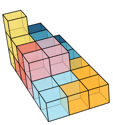
Solution for A426 enter image description here

The difficulty of these problems is probably higher than the Easy Cubes one. For the above solution of problem A426, I made two runs, using respectively ~88000 and 75000 iterations. This probably means that there is only a very small number of different solutions, and finding the solution is more time-consuming (typically between 10 minutes to a small multiple of it ?!). So the code given here should work for all the SOMA problems, but using a more advanced method (e.g. the dancing links algorithm by D. Knuth mentionned by Sander Huisman) would be a good idea if one needs all solutions of all problems... But anyway it is nice to see that a very naive method, quickly progammed, can give solutions.


Adapted code: definition of the pieces for SOMA problems (I did not make the effort to change the pieces names... the new pieces replace the definition of PLine, PSquare and PBulky, all the rest is unchanged)

Pieces Definitions
In[2]:= PTriangle = {{0, 0, 0}, {0, 1, 0}, {1, 0, 0}};
In[3]:= PSquare = {{0, 0, 0}, {0, 0, 1}, {1, 0, 0}, {1, -1, 0}};
In[4]:= PLine = {{0, 0, 0}, {1, 0, 0}, {0, 1, 0}, {0, 1, 1}};
In[5]:= PL = {{0, 0, 0}, {0, 1, 0}, {1, 0, 0}, {2, 0, 0}};
In[6]:= PPodium = {{0, 0, 0}, {0, 1, 0}, {-1, 0, 0}, {1, 0, 0}};
In[7]:= PSnake = {{0, 0, 0}, {0, 1, 0}, {1, 0, 0}, {-1, 1, 0}};
In[8]:= PBulky = {{0, 0, 0}, {1, 0, 0}, {0, -1, 0}, {0, 0, 1}};
In[9]:= (* Rotation by angle \[Pi]/2 matrix*)
In[10]:= Mrotz = {{0, 1, 0}, {-1, 0, 0}, {0, 0, 1}};
In[11]:= Mrotx = {{1, 0, 0}, {0, 0, 1}, {0, -1, 0}};
In[12]:= Mrotx = {{0, 0, -1}, {0, 1, 0}, {1, 0, 0}};
In[13]:= (* Reflection  matrix *)
In[14]:= Mrefx = {{-1, 0, 0}, {0, 1, 0}, {0, 0, 1}};
In[15]:= Mrefy = {{1, 0, 0}, {0, -1, 0}, {0, 0, 1}};
In[16]:= Mrefz = {{1, 0, 0}, {0, 1, 0}, {0, 0, -1}};
In[17]:= MUnit = {{1, 0, 0}, {0, 1, 0}, {0, 0, 1}};
In[18]:= (*Operators which peform a given number of rotation, and of \
reflection*)
In[19]:= RotatePiecex[piece_, n_] := Nest[Mrotx.# &, #, n] & /@ piece
In[20]:= RotatePiecey[piece_, n_] := Nest[Mrotx.# &, #, n] & /@ piece
In[21]:= RotatePiecez[piece_, n_] := Nest[Mrotz.# &, #, n] & /@ piece
In[22]:= ReflectPiecex[piece_, n_] := 
 If[n == 0, (MUnit.#) & /@ piece, (Mrefx.#) & /@ piece]
In[23]:= ReflectPiecey[piece_, n_] := 
 If[n == 0, (MUnit.#) & /@ piece, (Mrefy.#) & /@ piece]
In[24]:= ReflectPiecez[piece_, n_] := 
 If[n == 0, (MUnit.#) & /@ piece, (Mrefz.#) & /@ piece]
Each piece with all the possible orientations
In[25]:= MakeAllPieces[piece_] := 
 DeleteDuplicates@
  Table[Module[{Rota, Rotb, Rotc, Refa, Refb, Refc, na, nb, nc, ma, 
     mb, mc},
    Rota = RandomChoice[{RotatePiecex, RotatePiecey, RotatePiecez}];
    Rotb = RandomChoice[{RotatePiecex, RotatePiecey, RotatePiecez}]; 
    Rotc = RandomChoice[{RotatePiecex, RotatePiecey, RotatePiecez}];
    Refa = RandomChoice[{ReflectPiecex, ReflectPiecey, ReflectPiecez}];
    Refb = RandomChoice[{ReflectPiecex, ReflectPiecey, ReflectPiecez}];
    Refc = RandomChoice[{ReflectPiecex, ReflectPiecey, ReflectPiecez}];
    na = RandomInteger[{0, 3}]; nb = RandomInteger[{0, 3}]; 
    nc = RandomInteger[{0, 3}];
    ma = RandomInteger[{0, 1}]; mb = RandomInteger[{0, 1}]; 
    mc = RandomInteger[{0, 1}];
    Refc[Rotc[Refb[Rotb[ Refa[Rota[piece, na], ma], nb], mb], nc], 
     mc]], {i, 1, 2000}]
In[26]:= PTriangleAll = MakeAllPieces[PTriangle]; Length@PTriangleAll
Out[26]= 24
In[27]:= PSquareAll = MakeAllPieces[PSquare]; Length@PSquareAll
Out[27]= 48
In[28]:= PLineAll = MakeAllPieces[PLine]; Length@PLineAll
Out[28]= 48
In[29]:= PLAll = MakeAllPieces[PL]; Length@PLAll
Out[29]= 24
In[30]:= PPodiumAll = MakeAllPieces[PPodium]; Length@PPodiumAll
Out[30]= 24
In[31]:= PSnakeAll = MakeAllPieces[PSnake]; Length@PSnakeAll
Out[31]= 24
In[32]:= PBulkyAll = MakeAllPieces[PBulky]; Length@PBulkyAll
Out[32]= 48
In[33]:= tPieces = {PBulkyAll, PLAll, PPodiumAll, PSnakeAll, PSquareAll, 
   PLineAll, PTriangleAll};
In[34]:= tPiecesNames = {"Bu", "Ll", "Po", "Sn", "Sq", "Li", "Tr"};

Example of use on problem A

Solve problem A426 
In[71]:= coordA426 = 
 Join[Table[{0, j, 0}, {j, -3, 2}], Table[{1, j, 0}, {j, -3, 2}], 
  Table[{-1, j, 0}, {j, -3, 2}],
  Table[{0, j, 1}, {j, -1, 2}], Table[{-1, j, 1}, {j, -1, 2}], 
  Table[{-1, j, 2}, {j, 2, 2}]]
Out[71]= {{0, -3, 0}, {0, -2, 0}, {0, -1, 0}, {0, 0, 0}, {0, 1, 0}, {0, 2, 
  0}, {1, -3, 0}, {1, -2, 0}, {1, -1, 0}, {1, 0, 0}, {1, 1, 0}, {1, 2,
   0}, {-1, -3, 0}, {-1, -2, 0}, {-1, -1, 0}, {-1, 0, 0}, {-1, 1, 
  0}, {-1, 2, 0}, {0, -1, 1}, {0, 0, 1}, {0, 1, 1}, {0, 2, 
  1}, {-1, -1, 1}, {-1, 0, 1}, {-1, 1, 1}, {-1, 2, 1}, {-1, 2, 2}}
In[72]:= TheGridA426 = GridDefine[coordA426];
In[73]:= Plus @@ Flatten[ 1 - TheGridA426]
Out[73]= 27

In[75]:= SolgridA426ex1 = SolveGridBare[TheGridA426];
During evaluation of In[75]:= 88530
In[78]:= PlotGrid3D[SolgridA426ex1, All]

The "Easy cube" seems to be a simplified version of the "Soma cube". So, I wonder how easy would be to adapt the code given in this discussion for "Soma cube" constructs. E.g.

SOMA Figures A426450

POSTED BY: Anton Antonov

enter image description here - another post of yours has been selected for the Staff Picks group, congratulations !

We are happy to see you at the top of the "Featured Contributor" board. Thank you for your wonderful contributions, and please keep them coming!

POSTED BY: Moderation Team

I've seen a c++ code dancing links code for sudoku, it looked really complex. I'm quite sure it is not easy ;)

POSTED BY: Sander Huisman

Thank you for the info ! I did not know the dancing links algorithm. Having a look at the wikipedia page about it, it seems very interesting (and way more powerful than my basic algorithm). I have matter to study here.

Nicely done! I always wanted to program the dancing links algorithm that is used for 'exact cover' problems like this one! But your algorithm seems nice too. I'm gonna study it a bit!

POSTED BY: Sander Huisman
Reply to this discussion
Community posts can be styled and formatted using the Markdown syntax.
Reply Preview
Attachments
Remove
or Discard

Group Abstract Group Abstract