@Mike Sollami Thank you for digging into this.
In order to make Sabrina's code work again in v13, you can use the following definitions (before evaluating the layers/networks):
ScalarTimesLayer[s_] := ElementwiseLayer[s*#&]
UpsampleLayer[s_] := ResizeLayer[{Scaled[s], Scaled[s]}, Resampling->"Nearest"]
BroadcastPlusLayer[] := ThreadingLayer[Plus, InputPorts -> {"LHS", "RHS"}]
SplitLayer[False] := NetGraph[{PartLayer[1;;1], PartLayer[2;;2], PartLayer[3;;3]}, {}]
(Also remove suboption "Parallelize" -> False in NetEncoder[{"Image", ...}], and you can replace DotPlusLayer by LinearLayer to avoid warnings)
You also need to change, in the NetGraph edges:
..., "SplitL" -> {"LowLev", "TimesL1", "TimesL2"}, ...
by
..., NetPort["SplitL","Output1"] -> "LowLev",
NetPort["SplitL","Output2"] -> "TimesL1",
NetPort["SplitL","Output3"] -> "TimesL2", ...
Complete code:
$\[Alpha]=1/300;
$numClasses=4314;
ScalarTimesLayer[s_] := ElementwiseLayer[s*#&]
UpsampleLayer[s_] := ResizeLayer[{Scaled[s],Scaled[s]}, Resampling->"Nearest"]
BroadcastPlusLayer[] := ThreadingLayer[Plus, InputPorts -> {"LHS","RHS"}]
SplitLayer[False] := NetGraph[{PartLayer[1;;1],PartLayer[2;;2],PartLayer[3;;3]},{}]
conv[out_Integer,k_Integer,str_Integer,p_Integer]:=ConvolutionLayer[out,k,"Stride"->str,"PaddingSize"->p];(*Convolution layer*)
fc[n_Integer]:=LinearLayer[n];(*Fully connected layer*)
relu=ElementwiseLayer[Ramp];(*Ramp activation function*)
\[Sigma]=ElementwiseLayer[LogisticSigmoid];(*Sigmoid activation function*)
\[Sigma]1=ElementwiseLayer[LogisticSigmoid];
tl1=ScalarTimesLayer[100];(*This layer multiplies elementwise the input tensor by a scalar number*)
tl2=ScalarTimesLayer[100];
timesLoss=ScalarTimesLayer[$\[Alpha]];
bn=BatchNormalizationLayer[];(*Batch Normalizaion layer*)
upSampl=UpsampleLayer[2];(*Upsampling using the nearest neighbor techique*)
sl=SplitLayer[False];(*This layer splits the input tensor into its channels*)
cl=CatenateLayer[];(*This layer catenates the input tensors and outputs a new tensor*)
(*"Fusion" layer*)
rshL=ReshapeLayer[{256,1,1}];(*This layer reinterprets the input to be an array of the specified dimensions*)
bl=BroadcastPlusLayer[]; (*This layer catenates a vector all along the corresponding dimension of a tensor*)
(*Loss functions*)
lossMS=MeanSquaredLossLayer[];
lossCE=CrossEntropyLossLayer["Index"];
(* Low-Level Features Network *)
lln = NetChain[{conv[64, 3, 2, 1], bn, relu, conv[128, 3, 1, 1], bn, relu, conv[128, 3, 2, 1], bn, relu, conv[256, 3, 1, 1], bn, relu,
conv[256, 3, 2, 1], bn, relu, conv[512, 3, 1, 1], bn, relu} ];
(* Mid-Level Features Network *)
mln = NetChain[{conv[512, 3, 1, 1], bn, relu, conv[256, 3, 1, 1], bn, relu}];
(* Colorization Network *)
coln = NetChain[{conv[256, 3, 1, 1], bn, relu, conv[128, 3, 1, 1], bn, relu, upSampl, conv[64, 3, 1, 1], bn, relu, conv[64, 3, 1, 1],
bn, relu, upSampl, conv[32, 3, 1, 1], bn, relu, conv[2, 3, 1, 1], \[Sigma], upSampl}];
(* Global Features Network *)
gln = NetChain[{conv[512, 3, 2, 1], bn, relu, conv[512, 3, 1, 1], bn, relu, conv[512, 3, 2, 1], bn, relu, conv[512, 3, 1, 1], bn, relu,
FlattenLayer[], fc[1024], bn, relu, fc[512], bn, relu}];
gln2 = NetChain[{fc[256], bn, relu}];
(* Classification Network *)
classn = NetChain[{fc[256], bn, relu, fc[$numClasses], bn, relu}];
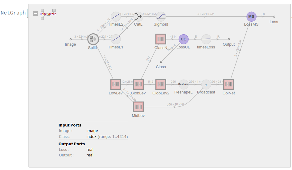
classNet = NetGraph[
<| "SplitL" -> sl, "LowLev" -> lln, "MidLev" -> mln, "GlobLev" -> gln, "GlobLev2" -> gln2, "ColNet" -> coln, "Sigmoid" -> \[Sigma]1, "TimesL1" -> tl1, "TimesL2" -> tl2, "CatL" -> cl,
"LossMS" -> lossMS, "LossCE" -> lossCE, "Broadcast" -> bl, "ReshapeL" -> rshL, "ClassN" -> classn, "timesLoss" -> timesLoss |>,
{ NetPort["Image"] -> "SplitL", NetPort["SplitL","Output1"] -> "LowLev", NetPort["SplitL","Output2"] -> "TimesL1", NetPort["SplitL","Output3"] -> "TimesL2", {"TimesL1", "TimesL2"} -> "CatL", "CatL" -> "Sigmoid",
"LowLev" -> "MidLev", "LowLev" -> "GlobLev", "GlobLev" -> "GlobLev2", "GlobLev" -> "ClassN", "MidLev" -> NetPort["Broadcast", "LHS"], "GlobLev2" -> "ReshapeL",
"ReshapeL" -> NetPort["Broadcast", "RHS"], "Broadcast" -> "ColNet", "ColNet" -> NetPort["LossMS", "Input"], "Sigmoid" -> NetPort["LossMS", "Target"], "ClassN" -> NetPort["LossCE", "Input"],
NetPort["Class"] -> NetPort["LossCE", "Target"], "LossCE" -> "timesLoss" },
"Image" -> NetEncoder[{"Image", {224, 224}, "ColorSpace" -> "LAB"}] ]