Message Boards Message Boards

[WSS16] Image Colorization

POSTED BY: Sabrina Giollo
17 Replies

It would be nice to see this work in v13. Here's an attempt to update the nonexistent functions from v11, check it out:

https://www.wolframcloud.com/obj/msollami/Published/colorization-2016.nb

There are only a few small changes that need to be made, for example:

(*upSampl = UpsampleLayer[2];*)
upSampl = ResizeLayer[{Scaled @ 2, Scaled @ 2}];
(* sl = SplitLayer[False]; *)
sl = TransposeLayer[3->1]; 
(* bl = BroadcastPlusLayer[]; *)
bl = CatenateLayer[InputPorts -> {"LHS", "RHS"}];

But the final NetGraph doesn't like them: enter image description here

This post is the only example of colorization that contains training/loss details, which are almost always missing from construction notebooks in WNNR. Let's help make this work again in v13...

POSTED BY: Michael Sollami

@Mike Sollami Thank you for digging into this.

In order to make Sabrina's code work again in v13, you can use the following definitions (before evaluating the layers/networks):

ScalarTimesLayer[s_] := ElementwiseLayer[s*#&]
UpsampleLayer[s_] := ResizeLayer[{Scaled[s], Scaled[s]}, Resampling->"Nearest"]
BroadcastPlusLayer[] := ThreadingLayer[Plus, InputPorts -> {"LHS", "RHS"}]
SplitLayer[False] := NetGraph[{PartLayer[1;;1], PartLayer[2;;2], PartLayer[3;;3]}, {}]

(Also remove suboption "Parallelize" -> False in NetEncoder[{"Image", ...}], and you can replace DotPlusLayer by LinearLayer to avoid warnings)

You also need to change, in the NetGraph edges:

..., "SplitL" -> {"LowLev", "TimesL1", "TimesL2"}, ...

by

..., NetPort["SplitL","Output1"] -> "LowLev",
NetPort["SplitL","Output2"] -> "TimesL1",
NetPort["SplitL","Output3"] -> "TimesL2", ...

Complete code:

$\[Alpha]=1/300;
$numClasses=4314;

ScalarTimesLayer[s_] := ElementwiseLayer[s*#&]
UpsampleLayer[s_] := ResizeLayer[{Scaled[s],Scaled[s]}, Resampling->"Nearest"]
BroadcastPlusLayer[] := ThreadingLayer[Plus, InputPorts -> {"LHS","RHS"}]
SplitLayer[False] := NetGraph[{PartLayer[1;;1],PartLayer[2;;2],PartLayer[3;;3]},{}]

conv[out_Integer,k_Integer,str_Integer,p_Integer]:=ConvolutionLayer[out,k,"Stride"->str,"PaddingSize"->p];(*Convolution layer*)
fc[n_Integer]:=LinearLayer[n];(*Fully connected layer*)
relu=ElementwiseLayer[Ramp];(*Ramp activation function*)
\[Sigma]=ElementwiseLayer[LogisticSigmoid];(*Sigmoid activation function*)
\[Sigma]1=ElementwiseLayer[LogisticSigmoid];
tl1=ScalarTimesLayer[100];(*This layer multiplies elementwise the input tensor by a scalar number*)
tl2=ScalarTimesLayer[100];
timesLoss=ScalarTimesLayer[$\[Alpha]];
bn=BatchNormalizationLayer[];(*Batch Normalizaion layer*)
upSampl=UpsampleLayer[2];(*Upsampling using the nearest neighbor techique*)
sl=SplitLayer[False];(*This layer splits the input tensor into its channels*)
cl=CatenateLayer[];(*This layer catenates the input tensors and outputs a new tensor*)

(*"Fusion" layer*)
rshL=ReshapeLayer[{256,1,1}];(*This layer reinterprets the input to be an array of the specified dimensions*)
bl=BroadcastPlusLayer[]; (*This layer catenates a vector all along the corresponding dimension of a tensor*)

(*Loss functions*)
lossMS=MeanSquaredLossLayer[];
lossCE=CrossEntropyLossLayer["Index"];

(* Low-Level Features Network *)
lln = NetChain[{conv[64, 3, 2, 1], bn, relu, conv[128, 3, 1, 1], bn, relu, conv[128, 3, 2, 1], bn, relu, conv[256, 3, 1, 1], bn, relu, 
    conv[256, 3, 2, 1], bn, relu, conv[512, 3, 1, 1], bn, relu} ];
(* Mid-Level Features Network *)
mln = NetChain[{conv[512, 3, 1, 1], bn, relu, conv[256, 3, 1, 1], bn, relu}];
(* Colorization Network *)
coln = NetChain[{conv[256, 3, 1, 1], bn, relu, conv[128, 3, 1, 1], bn, relu, upSampl, conv[64, 3, 1, 1], bn, relu, conv[64, 3, 1, 1], 
    bn, relu, upSampl, conv[32, 3, 1, 1], bn, relu, conv[2, 3, 1, 1], \[Sigma], upSampl}];
(* Global Features Network *)
gln = NetChain[{conv[512, 3, 2, 1], bn, relu, conv[512, 3, 1, 1], bn, relu, conv[512, 3, 2, 1], bn, relu, conv[512, 3, 1, 1], bn, relu, 
    FlattenLayer[], fc[1024], bn, relu, fc[512], bn, relu}];= NetChain[{fc[256], bn, relu}];
(* Classification Network *)
classn = NetChain[{fc[256], bn, relu, fc[$numClasses], bn, relu}];

classNet = NetGraph[
  <| "SplitL" -> sl, "LowLev" -> lln, "MidLev" -> mln, "GlobLev" -> gln, "GlobLev2" -> gln2, "ColNet" -> coln, "Sigmoid" -> \[Sigma]1, "TimesL1" -> tl1, "TimesL2" -> tl2, "CatL" -> cl,
  "LossMS" -> lossMS, "LossCE" -> lossCE, "Broadcast" -> bl, "ReshapeL" -> rshL, "ClassN" -> classn, "timesLoss" -> timesLoss |>,
  { NetPort["Image"] -> "SplitL", NetPort["SplitL","Output1"] -> "LowLev", NetPort["SplitL","Output2"] -> "TimesL1", NetPort["SplitL","Output3"] -> "TimesL2", {"TimesL1", "TimesL2"} -> "CatL", "CatL" -> "Sigmoid",
  "LowLev" -> "MidLev", "LowLev" -> "GlobLev", "GlobLev" -> "GlobLev2", "GlobLev" -> "ClassN", "MidLev" -> NetPort["Broadcast", "LHS"], "GlobLev2" -> "ReshapeL",
  "ReshapeL" -> NetPort["Broadcast", "RHS"], "Broadcast" -> "ColNet", "ColNet" -> NetPort["LossMS", "Input"], "Sigmoid" -> NetPort["LossMS", "Target"],  "ClassN" -> NetPort["LossCE", "Input"], 
   NetPort["Class"] -> NetPort["LossCE", "Target"], "LossCE" -> "timesLoss" }, 
  "Image" -> NetEncoder[{"Image", {224, 224}, "ColorSpace" -> "LAB"}] ]
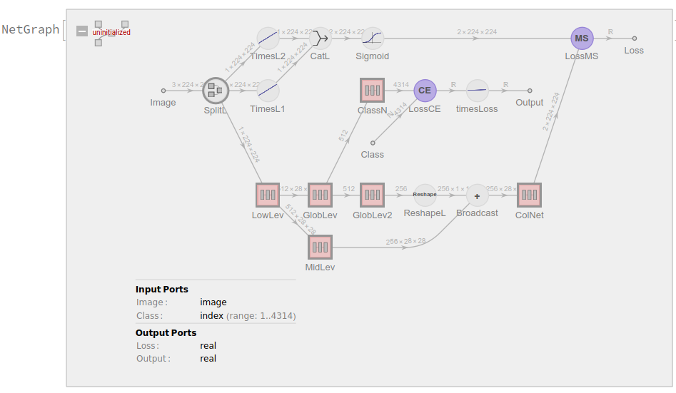
enter image description here

Are there any Wolfram Function Repository entries related to these kind of colorizations?

POSTED BY: Anton Antonov
POSTED BY: Michael Sollami

This one, no (for various reasons). A better one will be published very soon.

@Mike Sollami: There are two colorization nets available right now:

NetModel["ColorNet Image Colorization Trained on Places Data (Raw Model)"]

and

NetModel["ColorNet Image Colorization Trained on ImageNet Competition Data (Raw Model)"]

For usage, see here and here.

Posted 8 years ago

This is very interesting work! I have the NetChain from the discussion above and it looks fine and seems to work with a small training set. It is big training task to use the "Places" dataset and not really practical for the resources I have.

So my question - and this is really a question to Sebastian who mentioned it earlier in the discussion - could the trained network be made available?

POSTED BY: Steve Walker

There is an upcoming model gallery where this, and many more models will be available.

This is a good examples article for people who are interested in this project: http://www.thisisinsider.com/digitally-recolored-photos-2016-6

POSTED BY: Manjunath Babu
Posted 8 years ago

Thank you for your answer! Currently I'm testing the pre-release of Mathematica 11.0.0.0. My main objective is to see how you have implemented a network that looks so complex in Mathematica. It is not to run or train. This is why I have only asked for the Netchain. I understand that you probably can not post or send my email. Even so, thank you for sharing the great work that you have done!

POSTED BY: Luis Mendes

Global Variables

(* Loss function parameter and number of classes of the images *)
$\[Alpha] = 1/300;
$numClasses = 4314;

Net Layers

conv[out_Integer, k_Integer, str_Integer, p_Integer] := ConvolutionLayer[out, k, "Stride" -> str, "PaddingSize" -> p]; (* Convolution layer *)
fc[n_Integer] := DotPlusLayer[n]; (* Fully connected layer *)
relu = ElementwiseLayer[Ramp]; (* Ramp activation function *)
\[Sigma] = ElementwiseLayer[LogisticSigmoid];(* Sigmoid activation function *)
\[Sigma]1 = ElementwiseLayer[LogisticSigmoid];
tl1 = ScalarTimesLayer[100];  (* This layer multiplies elementwise the input tensor by a scalar number *)
tl2 = ScalarTimesLayer[100];
timesLoss = ScalarTimesLayer[$\[Alpha]];
bn = BatchNormalizationLayer[]; (* Batch Normalizaion layer *)
upSampl = UpsampleLayer[2]; (* Upsampling using the nearest neighbor techique *)
sl = SplitLayer[False];  (* This layer splits the input tensor into its channels *)     
cl = CatenateLayer[]; (* This layer catenates the input tensors and outputs a new tensor *)

(* "Fusion" layer *)
rshL = ReshapeLayer[{256, 1, 1}]; (* This layer reinterprets the input to be an array of the specified dimensions *)
bl = BroadcastPlusLayer[]; (* This layer catenates a vector all along the corresponding dimension of a tensor *)

(* Loss functions *)
lossMS = MeanSquaredLossLayer[]; 
lossCE = CrossEntropyLossLayer["Index"]; 

Net Chains

(* Low-Level Features Network *)
lln = NetChain[{conv[64, 3, 2, 1], bn, relu, conv[128, 3, 1, 1], bn, relu, conv[128, 3, 2, 1], bn, relu, conv[256, 3, 1, 1], bn, relu, 
    conv[256, 3, 2, 1], bn, relu, conv[512, 3, 1, 1], bn, relu} ];
(* Mid-Level Features Network *)
mln = NetChain[{conv[512, 3, 1, 1], bn, relu, conv[256, 3, 1, 1], bn, relu}];
(* Colorization Network *)
coln = NetChain[{conv[256, 3, 1, 1], bn, relu, conv[128, 3, 1, 1], bn, relu, upSampl, conv[64, 3, 1, 1], bn, relu, conv[64, 3, 1, 1], 
    bn, relu, upSampl, conv[32, 3, 1, 1], bn, relu, conv[2, 3, 1, 1], \[Sigma], upSampl}];
(* Global Features Network *)
gln = NetChain[{conv[512, 3, 2, 1], bn, relu, conv[512, 3, 1, 1], bn, relu, conv[512, 3, 2, 1], bn, relu, conv[512, 3, 1, 1], bn, relu, 
    FlattenLayer[], fc[1024], bn, relu, fc[512], bn, relu}];
gln2 = NetChain[{fc[256], bn, relu}];
(* Classification Network *)
classn = NetChain[{fc[256], bn, relu, fc[$numClasses], bn, relu}];

Net Structure

classNet = NetGraph[
  <| "SplitL" -> sl, "LowLev" -> lln, "MidLev" -> mln, "GlobLev" -> gln, "GlobLev2" -> gln2, "ColNet" -> coln, "Sigmoid" -> \[Sigma]1, "TimesL1" -> tl1, "TimesL2" -> tl2, "CatL" -> cl, "LossMS" -> lossMS, "LossCE" -> lossCE, "Broadcast" -> bl, "ReshapeL" -> rshL, "ClassN" -> classn, "timesLoss" -> timesLoss |>,
  { NetPort["Image"] -> "SplitL",  "SplitL" -> {"LowLev", "TimesL1", "TimesL2"}, {"TimesL1", "TimesL2"} -> "CatL", "CatL" -> "Sigmoid", "LowLev" -> "MidLev", "LowLev" -> "GlobLev", "GlobLev" -> "GlobLev2", "GlobLev" -> "ClassN", "MidLev" -> NetPort["Broadcast", "LHS"], "GlobLev2" -> "ReshapeL", "ReshapeL" -> NetPort["Broadcast", "RHS"], "Broadcast" -> "ColNet",
    "ColNet" -> NetPort["LossMS", "Input"], "Sigmoid" -> NetPort["LossMS", "Target"],  "ClassN" -> NetPort["LossCE", "Input"], 
   NetPort["Class"] -> NetPort["LossCE", "Target"], "LossCE" -> "timesLoss" }, 
  "Image" -> NetEncoder[{"Image", {224, 224}, "ColorSpace" -> "LAB", "Parallelize" -> False}] ]

Training

tnet = NetTrain [
  classNet,
  <|"Image" -> $trainPathsFile, "Class" -> $trainClasses|>,
  ValidationSet -> <|"Image" -> $testPathsFile, "Class" -> $testClasses|>,
  TargetDevice -> {"GPU", 1},
  "Method" -> "ADAM"
  ]

Evaluation Net

evalNet = Take[tnet, {"LowLev", "ColNet"}]
evalNet = NetChain[{evalNet}, "Input"->NetEncoder["Image",{224,224},"ColorSpace"->"Grayscale"]];
POSTED BY: Sabrina Giollo

Thanks for sharing, I was not really sure how to use the NetGraph, NetTrain, and NetChain, now it gives a bit more insight!

POSTED BY: Sander Huisman
Posted 8 years ago

Thank you!!!

POSTED BY: Luis Mendes
Posted 8 years ago

Great work!! It is possible you share the NetChain of the developed network?

POSTED BY: Luis Mendes

This network will only be runnable in the released version of M11.

Also: we are continuing to train the model (requires at least 2-3 weeks of training on a Titan X GPU for optimal performance, the images above were produced by a 14 hour trained net). If there is interest, I can post the trained net in 2 weeks time.

We are also working on a model gallery for 11.1 where we will post trained models like this one.

enter image description here - you earned "Featured Contributor" badge, congratulations !

This is a great post and it has been selected for the curated Staff Picks group. Your profile is now distinguished by a "Featured Contributor" badge and displayed on the "Featured Contributor" board.

POSTED BY: Moderation Team

Very impressive, thanks for sharing!

POSTED BY: Sander Huisman
Reply to this discussion
Community posts can be styled and formatted using the Markdown syntax.
Reply Preview
Attachments
Remove
or Discard

Group Abstract Group Abstract