I'd always wanted to make a 3D globe in Mathematica. Having only recently figured out how to go about it, and surprised by how little code it took to do, I've elected to share this nice little demo.

The heart of this implementation is the nifty function GeoElevationData[] (new in version 10), which allows one to generate an array of elevation values for any point on the Earth. From this, one can either choose to generate a relief map for textures, or as in the image above, an actual 3D globe.

To start off, here's the raw data to be used by the subsequent plots:

gdm = Reverse[QuantityMagnitude[GeoElevationData["World", "Geodetic", GeoZoomLevel -> 3, UnitSystem -> "Metric"]]];

(Increase the setting of GeoZoomLevel, or change the UnitSystem as seen fit.)

From this, one can use produce a quick visualization using ReliefPlot[], which could also be used as a nice texture:

ReliefPlot[gdm, BoxRatios -> {2, 1, 1/2}, ColorFunction -> "HypsometricTints", ColorFunctionScaling -> False, 
           DataRange -> {{-180, 180}, {-90, 90}}, Frame -> False, PlotRangePadding -> None]

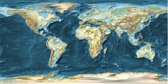
(I will note at this juncture that this is effectively what's being done behind the scenes when you use GeoStyling["ReliefMap"] in GeoGraphics[].)

But why be contented with a flat map, when we have actual elevation data! To make plotting slightly easier, build an interpolating function from the elevation data:

et = ListInterpolation[gdm, {{-90, 90}, {-180, 180}}];

With that, it is now a simple matter to generate a nice globe:

With[{s = 2*^5},
     ParametricPlot3D[(1 + et[?, ?]/s) {Cos[? °] Cos[? °],Cos[? °] Sin[? °], Sin[? °]}, {?, -180, 180}, {?, -90, 90},
                      Axes -> None, Boxed -> False, Mesh -> False, ColorFunctionScaling -> False,
                      ColorFunction -> (With[{r = Norm[{#1, #2, #3}]}, ColorData["HypsometricTints", s r - s]] &),
                      MaxRecursion -> 1, PlotPoints -> {1000, 500}, ViewPoint -> {-1.3, 2.4, 2.}]]

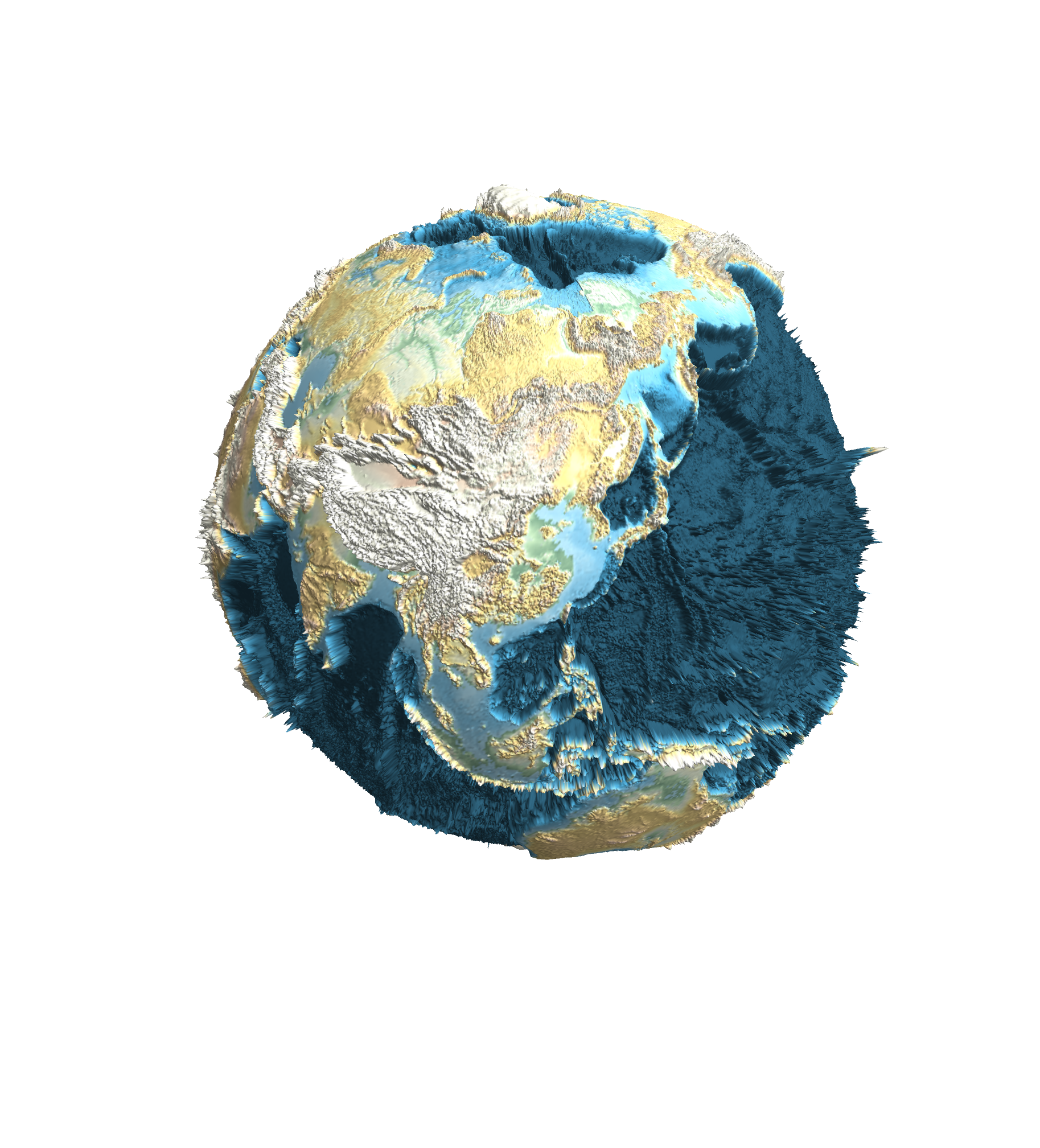
where I had chosen a scaling factor s that is smaller than the Earth's radius, to make the depressions and elevations slightly more prominent.

(Might be a bit hard to 3D-print, tho. Some smoothing and seam closing would be necessary)

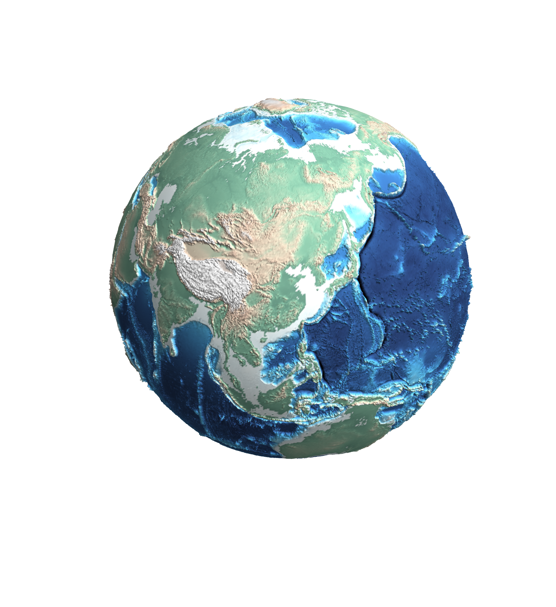
Not being contented with the default ColorData["HypsometricTints"], I decided to search for other nice color gradients. I found a few nice ones from cpt-city, but ultimately decided to synthesize my own using pieces of other gradients in that archive. The result was the following:

myGradient1 = Blend[{{-8000, RGBColor["#000000"]}, {-7000, RGBColor["#141E35"]}, {-6000, RGBColor["#263C6A"]},
                     {-5000, RGBColor["#2E5085"]}, {-4000, RGBColor["#3563A0"]}, {-3000, RGBColor["#4897D3"]},
                     {-2000, RGBColor["#5AB9E9"]}, {-1000, RGBColor["#8DD2EF"]}, {0, RGBColor["#F5FFFF"]},
                     {0, RGBColor["#699885"]}, {50, RGBColor["#76A992"]}, {200, RGBColor["#83B59B"]}, {600, RGBColor["#A5C0A7"]},
                     {1000, RGBColor["#D3C9B3"]}, {2000, RGBColor["#D4B8A4"]}, {3000, RGBColor["#DCDCDC"]},
                     {5000, RGBColor["#EEEEEE"]}, {6000, RGBColor["#F6F7F6"]}, {7000, RGBColor["#FAFAFA"]},
                     {8000, RGBColor["#FFFFFF"]}}, #] &;

Using this as the replacement for "HypsometricTints" as the ColorFunction yields the image at the beginning of my post.

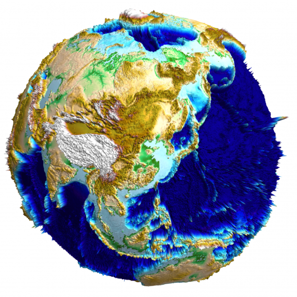
As a bonus image, I'd also found the colors needed to (more or less) reproduce ETOPO1; I'll omit them here, but show the resulting image (which some of you from Stack Exchange may have seen as my current Gravatar there):

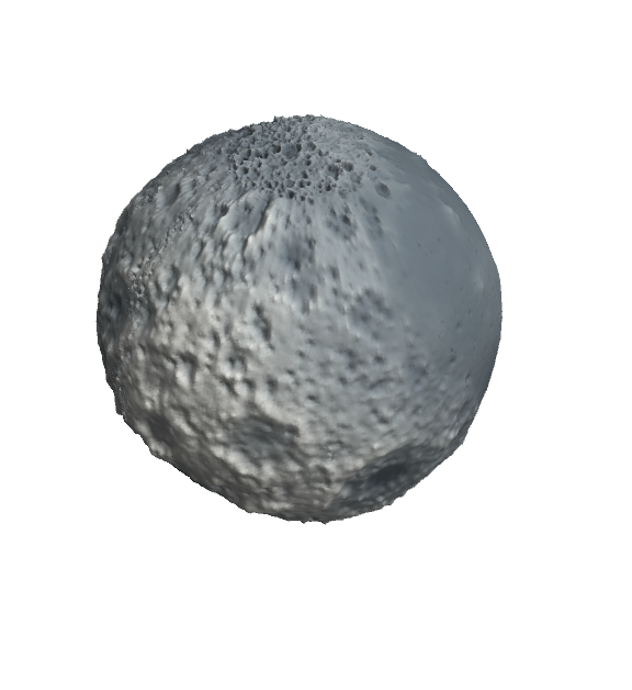
As a bonus bonus, one could also probably look up DEM data for other (terrestrial) planets and satellites, and render them using similar methods. I was able to generate a model of the Moon in this manner:

(I was prompted to post this, since Marco sorta kinda beat me to a nice and similar visualization in this thread. :D)